3.16: The Theory of Production

The Theory of Production

The theory of production examines the relationship between the factors of production (land, labor, capital, entrepreneur) and the output of goods and services. The theory of production is based on the "short run" or a period of production that allows production to change the amount of variable input, in this case, labor. The "long run" is a period of production that is long enough for producers to adjust various inputs to analyze the best mix of the factors of production.

Universal Generalizations

• The theory of production deals with the relationship between the factors of production and the output of goods and services.
• The law of variable proportions can explain how increasing units of a single input will cause the output to vary.

Guiding Questions

1. Why is it important for an owner of a company to understand the theory of production?
2. What is the easiest factor of production to change in order to vary total product output?

Video: Diminishing Marginal Returns

Video: Economies of Scale

Law of Variable Proportion

The Law of Variable Proportion can be best illustrated by using the "production function" for the concept that describes the relationship between changes in output to different amounts of a single input while all other inputs are held constant. This concept helps a producer determine the best use of resources to effect output. The basic model used by economists is the hypothetical production schedule to determine output when the number of workers changes. In this scenario, the company can calculate the total product, or total output, that the firm will produce.

Generally, there are three stages of production. Each stage impacts returns. Stage 1 begins when the first worker is hired, but there are not enough workers to produce efficiently enough to create a positive return. Until the company hires enough workers to run all of the machinery, this stage results in increasing returns. As long as each new worker contributes to the total output than the worker before, total output rises faster and faster.

Unfortunately, a company cannot continue in Stage 1 because as soon as it is discovered that adding additional workers increases output, the company continues to hire additional employees. By Stage 2 production output continues to rise, but at small and smaller increments. Soon additional workers hired may be needed to do things other than produce, like stock shelves or answer phones. The total production is slowing down so this stage is no longer producing increasing returns, but now it is diminishing returns.

At Stage 3 the company has hired too many workers and now the output is considered producing in negative returns. Too many workers get in each other's way and do not produce as much as in Stage 1 or even Stage 2. By Stage 3 the marginal output becomes negative and the total factory output decreases. The exact number of workers needed by a company can only be ascertained when the cost of adding each new worker is calculated. If the cost is low, then more workers can be hired. If the cost is high, the factory will need to consider how to produce the highest output amount in Stage 2 for the least amount of money.

Once the output has been calculated the measure is known as "marginal product". Marginal product is the extra output or change in the total product caused by the addition of one more unit of variable input, in this case, the number of workers. In order to determine the optimal input used in production, the changes in marginal product are examined in the various stages of production. The stages of production analyze the increasing returns, diminishing returns, and the negative returns, to calculate the best use of resources and inputs to produce at an optimal level.

How Production Costs Affect Supply

A supply curve shows how quantity supplied will change as the price rises and falls, assuming ceteris paribus so that no other economically relevant factors are changing. If other factors relevant to supply do change, then the entire supply curve will shift. Just as a shift in demand is represented by a change in the quantity demanded at every price, a shift in supply means a change in the quantity supplied at every price.

In thinking about the factors that affect supply, remember what motivates firms: profits, which are the difference between revenues and costs. Goods and services are produced using combinations of labor, materials, and machinery, or what we call inputs or factors of production. If a firm faces lower costs of production while the prices for the good or service the firm produces remain unchanged, a firm’s profits go up. When a firm’s profits increase, it is more motivated to produce output, since the more it produces the more profit it will earn. So, when costs of production fall, a firm will tend to supply a larger quantity at any given price for its output. This can be shown by the supply curve shifting to the right.

Take, for example, a messenger company that delivers packages around a city. The company may find that buying gasoline is one of its main costs. If the price of gasoline falls, then the company will find it can deliver messages more cheaply than before. Since lower costs correspond to higher profits, the messenger company may now supply more of its services at any given price. For example, given the lower gasoline prices, the company can now serve a greater area and increase its supply.

Conversely, if a firm faces higher costs of production, then it will earn lower profits at any given selling price for its products. As a result, a higher cost of production typically causes a firm to supply a smaller quantity at any given price. In this case, the supply curve shifts to the left.

Conversely, if a firm faces higher costs of production, then it will earn lower profits at any given selling price for its products. As a result, a higher cost of production typically causes a firm to supply a smaller quantity at any given price. In this case, the supply curve shifts to the left.

Consider the supply of cars, shown by curve S₀ in Figure 1. Point J indicates that if the price is $20,000, the quantity supplied will be 18 million cars. If the price rises to $22,000 per car, ceteris paribus, the quantity supplied will rise to 20 million cars, as point K on the S₀ curve shows. The same information can be shown in table form, as in Table 1.

Shifts in Supply: A Car Example

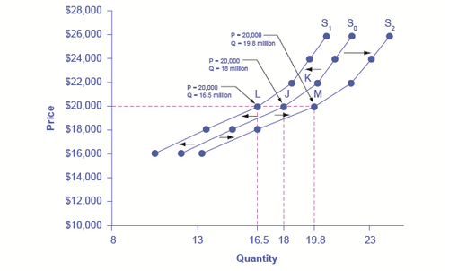
Decreased supply means that at every given price, the quantity supplied is lower, so that the supply curve shifts to the left, from S₀ to S₁. Increased supply means that at every given price, the quantity supplied is higher, so that the supply curve shifts to the right, from S₀ to S₂.

Price and Shifts in Supply: A Car Example

Price	Decrease to S1	Original Quantity Supplied S0	Increase to S2
$16,000	10.5 million	12.0 million	13.2 million
$18,000	13.5 million	15.0 million	16.5 million
$20,000	16.5 million	18.0 million	19.8 million
$22,000	18.5 million	20.0 million	22.0 million
$24,000	19.5 million	21.0 million	23.1 million
$26,000	20.5 million	22.0 million	24.2 million

Imagine that the price of steel, an important ingredient in manufacturing cars, rises. Now producing a car has become more expensive. At any given price for selling cars, car manufacturers will react by supplying a lower quantity. This can be shown graphically as a leftward shift of supply, from S₀ to S₁, which indicates that at any given price, the quantity supplied decreases. In this example, at a price of $20,000, the quantity supplied decreases from 18 million on the original supply curve (S₀) to 16.5 million on the supply curve S₁, which is labeled as point L.

Conversely, if the price of steel decreases, producing a car becomes less expensive. At any given price for selling cars, car manufacturers can now expect to earn higher profits, so they will supply a higher quantity. The shift of supply to the right, from S₀ to S₂, means that at all prices, the quantity supplied has increased. In this example, at a price of $20,000, the quantity supplied increases from 18 million on the original supply curve (S₀) to 19.8 million on the supply curve S₂, which is labeled M.

Economists often use the ceteris paribus or “other things being equal” assumption: while examining the economic impact of one event, all other factors remain unchanged for the purpose of the analysis. Factors that can shift the demand curve for goods and services, causing a different quantity to be demanded at any given price, include changes in tastes, population, income, prices of substitute or complement goods, and expectations about future conditions and prices. Factors that can shift the supply curve for goods and services, causing a different quantity to be supplied at any given price, include input prices, natural conditions, changes in technology, and government taxes, regulations, or subsidies.

Answer the self check questions below to monitor your understanding of the concepts in this section.

Self Check Questions

1. What is the theory of production?
2. The theory of production is generally based on the "short run". Which input is the variable that is changed? Why this one?
3. What does the Law of Variable Proportions state? Give an example of this law.
4. What is the production function? How can it be illustrated?
5. How many stages of production are there? Which stage is the best one to produce in?
6. Explain how marginal product changes in the stages of production.
7. What are diminishing returns?