
4.9: Monetary Policy, Banking and the Economy
- Page ID
- 1703
Monetary Policy, Banking & the Economy
The crucial question is how long will it take for the Fed’s policies to affect the economy? The influence of the Federal Reserve and monetary policy is enormous and complex. Not even the Fed can truly calculate exactly what will happen in the short-run or the long-run when it conducts monetary policy because there are various other issues to consider such as the timing and burden of that policy. When all the elements of the economic performance are analyzed and monetary policy is adjusted, the Fed may find the economy is difficult to “fine-tune”.
Universal Generalizations
- Changes in the money supply affect the interest rate, the availability of credit, and the price level.
- Expansion and contraction of the money supply affect the cost of credit.
- The quantity theory of money has been repeated throughout history.
Guiding Questions
- What is the short-run impact of monetary policy?
- Why do people view the interest rate as a measurement of the overall health of the economy?
- Why does the Fed try to avoid political confrontations, especially during election years?
 This table shows the different types of money commonly defined by economists. The bottom represents the most liquid forms of money, M0, which is used primarily as a means of exchange. The broadest measure of money defined here is M3. This includes forms of money used as a store of value.
Cash in your pocket certainly serves as money, but what about checks or credit cards? Are they money, too? Rather than trying to state a single way of measuring money, economists offer broader definitions of money based on liquidity. Liquidity refers to how quickly a financial asset can be used to buy a good or service. For example, cash is very liquid. Your $10 bill can be easily used to buy a hamburger at lunchtime. However, $10 that you have in your savings account is not so easy to use. You must go to the bank or ATM machine and withdraw that cash to buy your lunch. Thus, $10 in your savings account is less liquid.
Video: Fiscal and Monetary Policy
Measuring Money: Currency, M1, and M2
The Federal Reserve Bank, which is the central bank of the United States, is a bank regulator and is responsible for monetary policy and defines money according to its liquidity. There are two definitions of money: M1 and M2 money supply. M1 money supply includes those monies that are very liquid such as cash, checkable (demand) deposits, and traveler’s checks. M2 money supply is less liquid in nature and includes M1 plus savings and time deposits, certificates of deposits, and money market funds.
M1 money supply includes coins and currency in circulation—the coins and bills that circulate in an economy that are not held by the U.S. Treasury, at the Federal Reserve Bank, or in bank vaults. Closely related to currency are checkable deposits, also known as demand deposits. These are the amounts held in checking accounts. They are called demand deposits or checkable deposits because the banking institution must give the deposit holder his money “on demand” when a check is written or a debit card is used. These items together—currency, and checking accounts in banks—make up the definition of money known as M1, which is measured daily by the Federal Reserve System. Traveler’s checks are a also included in M1, but have decreased in use over the recent past.
A broader definition of money, M2 includes everything in M1 but also adds other types of deposits. For example, M2 includes savings deposits in banks, which are bank accounts on which you cannot write a check directly, but from which you can easily withdraw the money at an automatic teller machine or bank. Many banks and other financial institutions also offer a chance to invest in money market funds, where the deposits of many individual investors are pooled together and invested in a safe way, such as short-term government bonds. Another ingredient of M2 are the relatively small (that is, less than about $100,000) certificates of deposit (CDs) or time deposits, which are accounts that the depositor has committed to leaving in the bank for a certain period of time, ranging from a few months to a few years, in exchange for a higher interest rate. In short, all these types of M2 are money that you can withdraw and spend, but which require a greater effort to do so than the items in M1. Figure 2 should help in visualizing the relationship between M1 and M2. Note that M1 is included in the M2 calculation.
The Relationship Between M1 and M2 Money
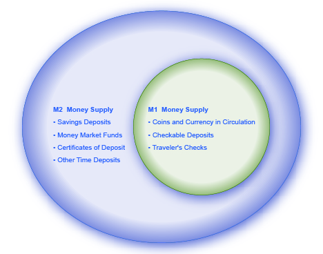
M1 and M2 money have several definitions, ranging from narrow to broad. M1 = coins and currency in circulation + checkable (demand) deposit + traveler’s checks. M2 = M1 + savings deposits + money market funds + certificates of deposit + other time deposits.
The Federal Reserve System is responsible for tracking the amounts of M1 and M2 and prepares a weekly release of information about the money supply. To provide an idea of what these amounts sound like, according to the Federal Reserve Bank’s measure of the U.S. money stock, at year-end 2012, M1 in the United States was $2.4 trillion, while M2 was $10.4 trillion. For comparison, the size of the U.S. GDP in 2012 was $16.3 trillion. A breakdown of the portion of each type of money that comprised M1 and M2 in 2012, as provided by the Federal Reserve Bank, is provided in Table 1.
| Components of M1 in the United States in 2012 | $ billions |
| Currency | $1,090.0 |
| Traveler’s checks | $3.8 |
| Demand deposits and other checking accounts | $1,351.1 |
| Total M1 | $2,444.9 (or $2.4 trillion) |
| Components of M2 in the United States in 2012 | $ billions |
| M1 money supply | $2,444.9 |
| Savings accounts | $6,692.0 |
| Time deposits | $631.0 |
| Individual money market mutual fund balances | $640.1 |
| Total M2 | $10,408.7 billion (or $10.4 trillion) |
The lines separating M1 and M2 can become a little blurry. Sometimes elements of M1 are not treated alike; for example, some businesses will not accept personal checks for large amounts, but will accept traveler’s checks or cash. Changes in banking practices and technology have made the savings accounts in M2 more similar to the checking accounts in M1. For example, some savings accounts will allow depositors to write checks, use automatic teller machines, and pay bills over the Internet, which has made it easier to access savings accounts. As with many other economic terms and statistics, the important point is to know the strengths and limitations of the various definitions of money, not to believe that such definitions are as clear-cut to economists as, say, the definition of nitrogen is to chemists.
Where does “plastic money” like debit cards, credit cards, and smart money fit into this picture? A debit card, like a check, is an instruction to the user’s bank to transfer money directly and immediately from your bank account to the seller. It is important to note that in our definition of money, it is checkable deposits that are money, not the paper check or the debit card. Although you can make a purchase with a credit card, it is not considered money but rather a short term loan from the credit card company to you. When you make a purchase with a credit card, the credit card company immediately transfers money from its checking account to the seller, and at the end of the month, the credit card company sends you a bill for what you have charged that month. Until you pay the credit card bill, you have effectively borrowed money from the credit card company. With a smart card, you can store a certain value of money on the card and then use the card to make purchases. Some “smart cards” used for specific purposes, like long-distance phone calls, or making purchases at a campus bookstore and cafeteria, are not really all that smart, because they can only be used for certain purchases or in certain places.
In short, credit cards, debit cards, and smart cards are different ways to move money when a purchase is made. But having more credit cards or debit cards does not change the quantity of money in the economy, any more than having more checks printed increases the amount of money in your checking account.
One key message underlying this discussion of M1 and M2 is that money in a modern economy is not just paper bills and coins; instead, money is closely linked to bank accounts. Indeed, the macroeconomic policies concerning money are largely conducted through the banking system. The next section explains how banks function and how a nation’s banking system has the power to create money.
Money is measured with several definitions: M1 includes currency and money in checking accounts (demand deposits). Traveler’s checks are also a component of M1, but are declining in use. M2 includes all of M1, plus savings deposits, time deposits like certificates of deposit, and money market funds.
The Problem of the Zero Percent Interest Rate Lower Bound
Most economists believe that monetary policy (the manipulation of interest rates and credit conditions by a nation’s central bank) has a powerful influence on a nation’s economy. Monetary policy works when the central bank reduces interest rates and makes credit more available. As a result, business investment and other types of spending increase, causing GDP and employment to grow.
But what if the interest rates banks pay are close to zero already? They cannot be made negative, can they? That would mean that lenders pay borrowers for the privilege of taking their money. Yet, this was the situation the U.S. Federal Reserve found itself in at the end of the 2008–2009 recession. The federal funds rate, which is the interest rate for banks that the Federal Reserve targets with its monetary policy, was slightly above 5% in 2007. By 2009, it had fallen to 0.16%.
The Federal Reserve’s situation was further complicated because fiscal policy, the other major tool for managing the economy, was constrained by fears that the federal budget deficit and the public debt were already too high. What were the Federal Reserve’s options? How could monetary policy be used to stimulate the economy? The answer, as we will see in this chapter, was to change the rules of the game.
Money, loans, and banks are all tied together. Money is deposited in bank accounts, which is then loaned to businesses, individuals, and other banks. When the interlocking system of money, loans, and banks works well, economic transactions are made smoothly in goods and labor markets and savers are connected with borrowers. If the money and banking system does not operate smoothly, the economy can either fall into recession or suffer prolonged inflation.
The government of every country has public policies that support the system of money, loans, and banking. But these policies do not always work perfectly. This chapter discusses how monetary policy works and what may prevent it from working perfectly.
How a Central Bank Executes Monetary Policy
The most important function of the Federal Reserve is to conduct the nation’s monetary policy. Article I, Section 8 of the U.S. Constitution gives Congress the power “to coin money” and “to regulate the value thereof.” As part of the 1913 legislation that created the Federal Reserve, Congress delegated these powers to the Fed. Monetary policy involves managing interest rates and credit conditions, which influences the level of economic activity, as described in more detail below.
A central bank has three traditional tools to implement monetary policy in the economy:
Open market operations
Changing reserve requirements
Changing the discount rate
In discussing how these three tools work, it is useful to think of the central bank as a “bank for banks”—that is, each private-sector bank has its own account at the central bank. We will discuss each of these monetary policy tools in the sections below.
Open Market Operations
The most commonly used tool of monetary policy in the U.S. is open market operations. Open market operations take place when the central bank sells or buys U.S. Treasury bonds in order to influence the quantity of bank reserves and the level of interest rates. The specific interest rate targeted in open market operations is the federal funds rate. The name is a bit of a misnomer since the federal funds rate is the interest rate charged by commercial banks making overnight loans to other banks. As such, it is a very short term interest rate, but one that reflects credit conditions in financial markets very well.
The Federal Open Market Committee (FOMC) makes the decisions regarding these open market operations. The FOMC is made up of the seven members of the Federal Reserve’s Board of Governors. It also includes five voting members who are drawn, on a rotating basis, from the regional Federal Reserve Banks. The New York district president is a permanent voting member of the FOMC and the other four spots are filled on a rotating, annual basis, from the other 11 districts. The FOMC typically meets every six weeks, but it can meet more frequently if necessary. The FOMC tries to act by consensus; however, the chairman of the Federal Reserve has traditionally played a very powerful role in defining and shaping that consensus. For the Federal Reserve, and for most central banks, open market operations have, over the last few decades, been the most commonly used tool of monetary policy.
To understand how open market operations affect the money supply, consider the balance sheet of Happy Bank, displayed in Figure 3. Figure 3 (a) shows that Happy Bank starts with $460 million in assets, divided among reserves, bonds and loans, and $400 million in liabilities in the form of deposits, with a net worth of $60 million. When the central bank purchases $20 million in bonds from Happy Bank, the bond holdings of Happy Bank fall by $20 million and the bank’s reserves rise by $20 million, as shown in Figure 3 (b). However, Happy Bank only wants to hold $40 million in reserves (the quantity of reserves that it started with in Figure 3) (a), so the bank decides to loan out the extra $20 million in reserves and its loans rise by $20 million, as shown in Figure 3 (c). The open market operation by the central bank causes Happy Bank to make loans instead of holding its assets in the form of government bonds, which expands the money supply. As the new loans are deposited in banks throughout the economy, these banks will, in turn, loan out some of the deposits they receive, triggering the money multiplier.
Balance Sheet of Happy Bank - Version 1
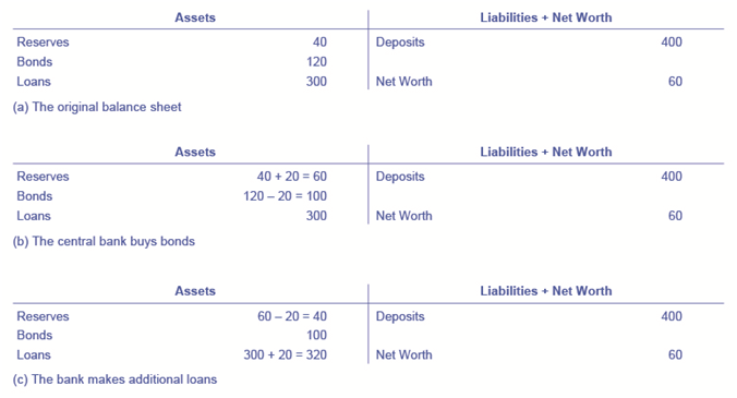
Where did the Federal Reserve get the $20 million that it used to purchase the bonds? A central bank has the power to create money. In practical terms, the Federal Reserve would write a check to Happy Bank, so that Happy Bank can have that money credited to its bank account at the Federal Reserve. In truth, the Federal Reserve created the money to purchase the bonds out of thin air—or with a few clicks on some computer keys.
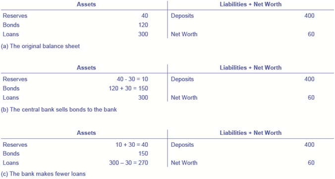
Open market operations can also reduce the quantity of money and loans in an economy. Figure 3 (a) shows the balance sheet of Happy Bank before the central bank sells bonds in the open market. When Happy Bank purchases $30 million in bonds, Happy Bank sends $30 million of its reserves to the central bank, but now holds an additional $30 million in bonds, as shown in Figure 4 (b). However, Happy Bank wants to hold $40 million in reserves, as in Figure 3 (a), so it will adjust down the quantity of its loans by $30 million, to bring its reserves back to the desired level, as shown in Figure 4 (c). In practical terms, a bank can easily reduce its quantity of loans. At any given time, a bank is receiving payments on loans that it made previously and also making new loans. If the bank just slows down or briefly halts making new loans, and instead adds those funds to its reserves, then its overall quantity of loans will decrease. A decrease in the quantity of loans also means fewer deposits in other banks, and other banks reducing their lending as well, as the money multiplier takes effect. And what about all those bonds? How do they affect the money supply? Read the following for the answer.
Balance Sheet of Happy Bank - Version 2
Does Selling or Buying Bonds Increase the Money Supply?
Is it a sale of bonds by the central bank which increases bank reserves and lowers interest rates or is it a purchase of bonds by the central bank? The easy way to keep track of this is to treat the central bank as being outside the banking system. When a central bank buys bonds, money is flowing from the central bank to individual banks in the economy, increasing the supply of money in circulation. When a central bank sells bonds, then money from individual banks in the economy is flowing into the central bank—reducing the quantity of money in the economy.
Changing Reserve Requirements
A second method of conducting monetary policy is for the central bank to raise or lower the reserve requirement, which, as noted earlier, is the percentage of each bank’s deposits that it is legally required to hold either as cash in their vault or on deposit with the central bank. If banks are required to hold a greater amount in reserves, they have less money available to lend out. If banks are allowed to hold a smaller amount in reserves, they will have a greater amount of money available to lend out.
At the end of 2013, the Federal Reserve required banks to hold reserves equal to 0% of the first $13.3 million in deposits, then to hold reserves equal to 3% of the deposits up to $89.0 million in checking and savings accounts, and 10% of any amount above $89.0 million. Small changes in the reserve requirements are made almost every year. For example, the $89.0 million dividing line is sometimes bumped up or down by a few million dollars. In practice, large changes in reserve requirements are rarely used to execute monetary policy. A sudden demand that all banks increase their reserves would be extremely disruptive and difficult to comply with, while loosening requirements too much would create a danger of banks being unable to meet the demand for withdrawals.
Changing the Discount Rate
The Federal Reserve was founded in the aftermath of the Financial Panic of 1907 when many banks failed as a result of bank runs. As mentioned earlier, since banks make profits by lending out their deposits, no bank, even those that are not bankrupt, can withstand a bank run. As a result of the Panic, the Federal Reserve was founded to be the “lender of last resort.” In the event of a bank run, sound banks, (banks that were not bankrupt) could borrow as much cash as they needed from the Fed’s discount “window” to quell the bank run. The interest rate banks pay for such loans is called the discount rate. (They are so named because loans are made against the bank’s outstanding loans “at a discount” of their face value.) Once depositors became convinced that the bank would be able to honor their withdrawals, they no longer had a reason to make a run on the bank. In short, the Federal Reserve was originally intended to provide credit passively, but in the years since its founding, the Fed has taken on a more active role with monetary policy.
So, the third traditional method for conducting monetary policy is to raise or lower the discount rate. If the central bank raises the discount rate, then commercial banks will reduce their borrowing of reserves from the Fed, and instead call in loans to replace those reserves. Since fewer loans are available, the money supply falls and market interest rates rise. If the central bank lowers the discount rate it charges to banks, the process works in reverse.
In recent decades, the Federal Reserve has made relatively few discount loans. Before a bank borrows from the Federal Reserve to fill out its required reserves, the bank is expected to first borrow from other available sources, like other banks. This is encouraged by Fed’s charging a higher discount rate, than the federal funds rate. Given that most banks borrow little at the discount rate, changing the discount rate up or down has little impact on their behavior. More importantly, the Fed has found from experience that open market operations are a more precise and powerful means of executing any desired monetary policy.
In the Federal Reserve Act, the phrase “...to afford means of rediscounting commercial paper” is contained in its long title. This tool was seen as the main tool for monetary policy when the Fed was initially created. This illustrates how monetary policy has evolved and how it continues to do so.
A central bank has three traditional tools to conduct monetary policy: open market operations, which involves buying and selling government bonds with banks; reserve requirements, which determine what level of reserves a bank is legally required to hold; and discount rates, which is the interest rate charged by the central bank on the loans that it gives to other commercial banks. The most commonly used tool is open market operations.
Monetary Policy and Economic Outcomes
A monetary policy that lowers interest rates and stimulates borrowing is known as an expansionary monetary policy or loose monetary policy. Conversely, a monetary policy that raises interest rates and reduces borrowing in the economy is a contractionary monetary policy or tight monetary policy. This module will discuss how expansionary and contractionary monetary policies affect interest rates and aggregate demand, and how such policies will affect macroeconomic goals like unemployment and inflation. We will conclude with a look at the Fed’s monetary policy practice in recent decades.
The Effect of Monetary Policy on Interest Rates
Consider the market for loanable bank funds, shown in Figure 5. The original equilibrium (E0) occurs at an interest rate of 8% and a quantity of funds loaned and borrowed of $10 billion. An expansionary monetary policy will shift the supply of loanable funds to the right from the original supply curve (S0) to S1, leading to an equilibrium (E1) with a lower interest rate of 6% and a quantity of funds loaned of $14 billion. Conversely, a contractionary monetary policy will shift the supply of loanable funds to the left from the original supply curve (S0) to S2, leading to an equilibrium (E2) with a higher interest rate of 10% and a quantity of funds loaned of $8 billion.
Monetary Policy and Interest Rates
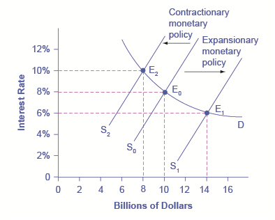
The original equilibrium occurs at E0. An expansionary monetary policy will shift the supply of loanable funds to the right from the original supply curve (S0) to the new supply curve (S1) and to a new equilibrium of E1, reducing the interest rate from 8% to 6%. A contractionary monetary policy will shift the supply of loanable funds to the left from the original supply curve (S0) to the new supply (S2), and raise the interest rate from 8% to 10%.
So how does a central bank “raise” interest rates? When describing the monetary policy actions taken by a central bank, it is common to hear that the central bank “raised interest rates” or “lowered interest rates.” We need to be clear about this: more precisely, through open market operations the central bank changes bank reserves in a way which affects the supply curve of loanable funds. As a result, interest rates change, as shown in Figure 5. If they do not meet the Fed’s target, the Fed can supply more or less reserves until interest rates do.
Recall that the specific interest rate the Fed targets is the federal funds rate. The Federal Reserve has, since 1995, established its target federal funds rate in advance of any open market operations.
Of course, financial markets display a wide range of interest rates, representing borrowers with different risk premiums and loans that are to be repaid over different periods of time. In general, when the federal funds rate drops substantially, other interest rates drop, too, and when the federal funds rate rises, other interest rates rise. However, a fall or rise of one percentage point in the federal funds rate—which remember is for borrowing overnight—will typically have an effect of less than one percentage point on a 30-year loan to purchase a house or a three-year loan to purchase a car. Monetary policy can push the entire spectrum of interest rates higher or lower, but the specific interest rates are set by the forces of supply and demand in those specific markets for lending and borrowing.
The Effect of Monetary Policy on Aggregate Demand
Monetary policy affects interest rates and the available quantity of loanable funds, which in turn affects several components of aggregate demand. Tight or contractionary monetary policy that leads to higher interest rates and a reduced quantity of loanable funds will reduce two components of aggregate demand. Business investment will decline because it is less attractive for firms to borrow money, and even firms that have money will notice that, with higher interest rates, it is relatively more attractive to put those funds in a financial investment than to make an investment in physical capital. In addition, higher interest rates will discourage consumer borrowing for big-ticket items like houses and cars. Conversely, loose or expansionary monetary policy that leads to lower interest rates and a higher quantity of loanable funds will tend to increase business investment and consumer borrowing for big-ticket items.
If the economy is suffering a recession and high unemployment, with output below potential GDP, expansionary monetary policy can help the economy return to potential GDP. Figure 6 (a) illustrates this situation. This example uses a short-run upward-sloping Keynesian aggregate supply curve (SRAS). The original equilibrium during a recession of E0 occurs at an output level of 600. An expansionary monetary policy will reduce interest rates and stimulate investment and consumption spending, causing the original aggregate demand curve (AD0) to shift right to AD1, so that the new equilibrium (E1) occurs at the potential GDP level of 700.
Expansionary or Contractionary Monetary Policy
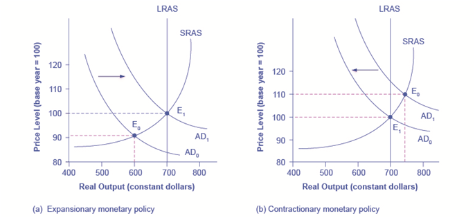
(a) The economy is originally in a recession with the equilibrium output and price level shown at E0. Expansionary monetary policy will reduce interest rates and shift aggregate demand to the right from AD0 to AD1, leading to the new equilibrium (E1) at the potential GDP level of output with a relatively small rise in the price level. (b) The economy is originally producing above the potential GDP level of output at the equilibrium E0 and is experiencing pressures for an inflationary rise in the price level. Contractionary monetary policy will shift aggregate demand to the left from AD0 to AD1, thus leading to a new equilibrium (E1) at the potential GDP level of output.
Conversely, if an economy is producing at a quantity of output above its potential GDP, a contractionary monetary policy can reduce the inflationary pressures for a rising price level. In Figure 6 (b), the original equilibrium (E0) occurs at an output of 750, which is above potential GDP. A contractionary monetary policy will raise interest rates, discourage borrowing for investment and consumption spending, and cause the original demand curve (AD0) to shift left to AD1, so that the new equilibrium (E1) occurs at the potential GDP level of 700.
These examples suggest that monetary policy should be countercyclical; that is, it should act to counterbalance the business cycles of economic downturns and upswings. Monetary policy should be loosened when a recession has caused unemployment to increase and tightened when inflation threatens. Of course, countercyclical policy does pose a danger of overreaction. If loose monetary policy seeking to end a recession goes too far, it may push aggregate demand so far to the right that it triggers inflation. If tight monetary policy seeking to reduce inflation goes too far, it may push aggregate demand so far to the left that a recession begins. Figure 7 (a) summarizes the chain of effects that connect loose and tight monetary policy to changes in output and the price level.
The Pathways of Monetary Policy
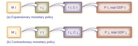
(a) In expansionary monetary policy the central bank causes the supply of money and loanable funds to increase, which lowers the interest rate, stimulating additional borrowing for investment and consumption, and shifting aggregate demand right. The result is a higher price level and, at least in the short run, higher real GDP. (b) In contractionary monetary policy, the central bank causes the supply of money and credit in the economy to decrease, which raises the interest rate, discouraging borrowing for investment and consumption, and shifting aggregate demand left. The result is a lower price level and, at least in the short run, lower real GDP.
Federal Reserve Actions Over Last Four Decades
For the period from the mid-1970s up through the end of 2007, Federal Reserve monetary policy can largely be summed up by looking at how it targeted the federal funds interest rate using open market operations.
Of course, telling the story of the U.S. economy since 1975 in terms of Federal Reserve actions leaves out many other macroeconomic factors that were influencing unemployment, recession, economic growth, and inflation over this time. The nine episodes of Federal Reserve action outlined in the sections below also demonstrate that the central bank should be considered one of the leading actors influencing the macro economy. As noted earlier, the single person with the greatest power to influence the U.S. economy is probably the chairperson of the Federal Reserve.
Figure 8 shows how the Federal Reserve has carried out monetary policy by targeting the federal funds interest rate in the last few decades. The graph shows the federal funds interest rate (remember, this interest rate is set through open market operations), the unemployment rate, and the inflation rate since 1975. Different episodes of monetary policy during this period are indicated in the figure.
Monetary Policy, Unemployment, and Inflation
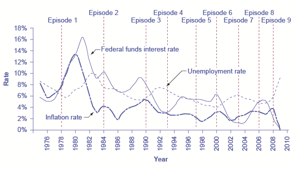
Through the episodes shown here, the Federal Reserve typically reacted to higher inflation with a contractionary monetary policy and a higher interest rate, and reacted to higher unemployment with an expansionary monetary policy and a lower interest rate.
Episode 1
Consider Episode 1 in the late 1970s. The rate of inflation was very high, exceeding 10% in 1979 and 1980, so the Federal Reserve used tight monetary policy to raise interest rates, with the federal funds rate rising from 5.5% in 1977 to 16.4% in 1981. By 1983, inflation was down to 3.2%, but aggregate demand contracted sharply enough that back-to-back recessions occurred in 1980 and in 1981–1982, and the unemployment rate rose from 5.8% in 1979 to 9.7% in 1982.
Episode 2
In Episode 2, in the early 1980s when the Federal Reserve was persuaded that inflation was declining, the Fed began slashing interest rates to reduce unemployment. The federal funds interest rate fell from 16.4% in 1981 to 6.8% in 1986. By 1986 or so, inflation had fallen to about 2% and the unemployment rate had come down to 7%, and was still falling.
Episode 3
In Episode 3, however, in the late 1980s, inflation appeared to be creeping up again, rising from 2% in 1986 up toward 5% by 1989. In response, the Federal Reserve used contractionary monetary policy to raise the federal funds rates from 6.6% in 1987 to 9.2% in 1989. The tighter monetary policy stopped inflation, which fell from above 5% in 1990 to under 3% in 1992, but it also helped to cause the recession of 1990–1991, and the unemployment rate rose from 5.3% in 1989 to 7.5% by 1992.
Episode 4
In Episode 4, in the early 1990s, when the Federal Reserve was confident that inflation was back under control, it reduced interest rates, with the federal funds interest rate falling from 8.1% in 1990 to 3.5% in 1992. As the economy expanded, the unemployment rate declined from 7.5% in 1992 to less than 5% by 1997.
Episodes 5 and 6
In Episodes 5 and 6, the Federal Reserve perceived a risk of inflation and raised the federal funds rate from 3% to 5.8% from 1993 to 1995. Inflation did not rise, and the period of economic growth during the 1990s continued. Then in 1999 and 2000, the Fed was concerned that inflation seemed to be creeping up so it raised the federal funds interest rate from 4.6% in December 1998 to 6.5% in June 2000. By early 2001, inflation was declining again, but a recession occurred in 2001. Between 2000 and 2002, the unemployment rate rose from 4.0% to 5.8%.
Episodes 7 and 8
In Episodes 7 and 8, the Federal Reserve conducted a loose monetary policy and slashed the federal funds rate from 6.2% in 2000 to just 1.7% in 2002, and then again to 1% in 2003. They actually did this because of fear of Japan-style deflation; this persuaded them to lower the Fed funds further than they otherwise would have. The recession ended, but, unemployment rates were slow to decline in the early 2000s. Finally, in 2004, the unemployment rate declined and the Federal Reserve began to raise the federal funds rate until it reached 5% by 2007.
Episode 9
In Episode 9, as the Great Recession took hold in 2008, the Federal Reserve was quick to slash interest rates, taking them down to 2% in 2008 and to nearly 0% in 2009. When the Fed had taken interest rates down to near-zero by December 2008, the economy was still deep in recession. Open market operations could not make the interest rate turn negative. The Federal Reserve had to think “outside the box.”
Quantitative Easing
The most powerful and commonly used of the three traditional tools of monetary policy—open market operations—works by expanding or contracting the money supply in a way that influences the interest rate. In late 2008, as the U.S. economy struggled with recession, the Federal Reserve had already reduced the interest rate to near-zero. With the recession still ongoing, the Fed decided to adopt an innovative and nontraditional policy known as quantitative easing (QE). This is the purchase of long-term government and private mortgage-backed securities by central banks to make credit available so as to stimulate aggregate demand.
Quantitative easing differed from traditional monetary policy in several key ways. First, it involved the Fed purchasing long term Treasury bonds, rather than short term Treasury bills. In 2008, however, it was impossible to stimulate the economy any further by lowering short term rates because they were already as low as they could get. (Read the closing Bring it Home feature for more on this.) Therefore, Bernanke sought to lower long-term rates utilizing quantitative easing.
This leads to a second way QE is different from traditional monetary policy. Instead of purchasing Treasury securities, the Fed also began purchasing private mortgage-backed securities, something it had never done before. During the financial crisis, which precipitated the recession, mortgage-backed securities were termed “toxic assets,” because when the housing market collapsed, no one knew what these securities were worth, which put the financial institutions which were holding those securities on very shaky ground. By offering to purchase mortgage-backed securities, the Fed was both pushing long term interest rates down and also removing possibly “toxic assets” from the balance sheets of private financial firms, which would strengthen the financial system.
Quantitative easing (QE) occurred in three episodes:
- During QE1, which began in November 2008, the Fed purchased $600 billion in mortgage-backed securities from government enterprises Fannie Mae and Freddie Mac.
- In November 2010, the Fed began QE2, in which it purchased $600 billion in U.S. Treasury bonds.
- QE3, began in September 2012 when the Fed commenced purchasing $40 billion of additional mortgage-backed securities per month. This amount was increased in December 2012 to $85 billion per month. The Fed has stated that, when economic conditions permit, it will begin tapering (or reducing the monthly purchases). This has not yet happened as of early 2014.
The quantitative easing policies adopted by the Federal Reserve (and by other central banks around the world) are usually thought of as temporary emergency measures. If these steps are, indeed, to be temporary, then the Federal Reserve will need to stop making these additional loans and sell off the financial securities it has accumulated. The concern is that the process of quantitative easing may prove more difficult to reverse than it was to enact. The evidence suggests that QE1 was somewhat successful, but that QE2 and QE3 have been less so.
An expansionary (or loose) monetary policy raises the quantity of money and credit above what it otherwise would have been and reduces interest rates, boosting aggregate demand, and thus countering recession. A contractionary monetary policy, also called a tight monetary policy, reduces the quantity of money and credit below what it otherwise would have been and raises interest rates, seeking to hold down inflation. During the 2008–2009 recession, central banks around the world also used quantitative easing to expand the supply of credit.
Pitfalls for Monetary Policy
In the real world, effective monetary policy faces a number of significant hurdles. Monetary policy affects the economy only after a time lag that is typically long and of variable length. Remember, monetary policy involves a chain of events: the central bank must perceive a situation in the economy, hold a meeting, and make a decision to react by tightening or loosening monetary policy. The change in monetary policy must percolate through the banking system, changing the quantity of loans and affecting interest rates. When interest rates change, businesses must change their investment levels and consumers must change their borrowing patterns when purchasing homes or cars. Then it takes time for these changes to filter through the rest of the economy.
As a result of this chain of events, monetary policy has little effect in the immediate future; instead, its primary effects are felt perhaps one to three years in the future. The reality of long and variable time lags does not mean that a central bank should refuse to make decisions. It does mean that central banks should be humble about taking action, because of the risk that their actions can create as much or more economic instability as they resolve.
Excess Reserves
Banks are legally required to hold a minimum level of reserves, but no rule prohibits them from holding additional excess reserves above the legally mandated limit. For example, during a recession banks may be hesitant to lend, because they fear that when the economy is contracting, a high proportion of loan applicants become less likely to repay their loans.
When many banks are choosing to hold excess reserves, expansionary monetary policy may not work well. This may occur because the banks are concerned about a deteriorating economy, while the central bank is trying to expand the money supply. If the banks prefer to hold excess reserves above the legally required level, the central bank cannot force individual banks to make loans. Similarly, sensible businesses and consumers may be reluctant to borrow substantial amounts of money in a recession, because they recognize that firms’ sales and employees’ jobs are more insecure in a recession, and they do not want to face the need to make interest payments. The result is that during an especially deep recession, an expansionary monetary policy may have little effect on either the price level or the real GDP.
Japan experienced this situation in the 1990s and early 2000s. Japan’s economy entered a period of very slow growth, dipping in and out of recession, in the early 1990s. By February 1999, the Bank of Japan had lowered the equivalent of its federal funds rate to 0%. It kept it there most of the time through 2003. Moreover, in the two years from March 2001 to March 2003, the Bank of Japan also expanded the money supply of the country by about 50%—an enormous increase. Even this highly expansionary monetary policy, however, had no substantial effect on stimulating aggregate demand. Japan’s economy continued to experience extremely slow growth into the mid-2000s.
Unpredictable Movements of Velocity
Velocity is a term that economists use to describe how quickly money circulates through the economy. The velocity of money in a year is defined as:
Velocity = nominal GDP
money supply
Specific measurements of velocity depend on the definition of the money supply being used. Consider the velocity of M1, the total amount of currency in circulation and checking account balances. In 2009, for example, M1 was $1.7 trillion and nominal GDP was $14.3 trillion, so the velocity of M1 was 8.4 ($14.3 trillion/$1.7 trillion). A higher velocity of money means that the average dollar circulates more times in a year; a lower velocity means that the average dollar circulates fewer times in a year.
Perhaps you heard the “d” word mentioned during our recent economic downturn. See the following Clear It Up feature for a discussion of how deflation could affect monetary policy.
What Happens During Episodes of Deflation?
Deflation occurs when the rate of inflation is negative; that is, instead of money having less purchasing power over time, as occurs with inflation, money is worth more. Deflation can make it very difficult for monetary policy to address a recession.
Remember that the real interest rate is the nominal interest rate minus the rate of inflation. If the nominal interest rate is 7% and the rate of inflation is 3%, then the borrower is effectively paying a 4% real interest rate. If the nominal interest rate is 7% and there is deflation of 2%, then the real interest rate is actually 9%. In this way, an unexpected deflation raises the real interest payments for borrowers. It can lead to a situation where an unexpectedly high number of loans are not repaid, and banks find that their net worth is decreasing or negative. When banks are suffering losses, they become less able and eager to make new loans. Aggregate demand declines, which can lead to recession.
Then the double-whammy: After causing a recession, deflation can make it difficult for monetary policy to work. Say that the central bank uses expansionary monetary policy to reduce the nominal interest rate all the way to zero—but the economy has 5% deflation. As a result, the real interest rate is 5%, and because a central bank cannot make the nominal interest rate negative, an expansionary policy cannot reduce the real interest rate further.
In the U.S. economy during the early 1930s, deflation was 6.7% per year from 1930–1933, which caused many borrowers to default on their loans and many banks to end up bankrupt, which in turn contributed substantially to the Great Depression. Not all episodes of deflation, however, end in economic depression. Japan, for example, experienced deflation of slightly less than 1% per year from 1999–2002, which hurt the Japanese economy, but it still grew by about 0.9% per year over this period. Indeed, there is at least one historical example of deflation coexisting with rapid growth. The U.S. economy experienced deflation of about 1.1% per year over the quarter-century from 1876–1900, but real GDP also expanded at a rapid clip of 4% per year over this time, despite some occasional severe recessions.
The central bank should be on guard against deflation and, if necessary, use expansionary monetary policy to prevent any long-lasting or extreme deflation from occurring. Except in severe cases like the Great Depression, deflation does not guarantee economic disaster.
Changes in velocity can cause problems for monetary policy. To understand why, rewrite the definition of velocity so that the money supply is on the left-hand side of the equation. That is:
- Recall that
- Nominal GDP = Price Level (or GDP Deflator) x Real GDP.
- Therefore,
- Money Supply x velocity = Nominal GDP = Price Level x Real GDP.
This equation is sometimes called the basic quantity equation of money but, as you can see, it is just the definition of velocity written in a different form. This equation must hold true, by definition.
If velocity is constant over time, then a certain percentage rise in the money supply on the left-hand side of the basic quantity equation of money will inevitably lead to the same percentage rise in nominal GDP—although this change could happen through an increase in inflation, or an increase in real GDP, or some combination of the two. If velocity is changing over time but in a constant and predictable way, then changes in the money supply will continue to have a predictable effect on nominal GDP. If velocity changes unpredictably over time, however, then the effect of changes in the money supply on nominal GDP becomes unpredictable.
The actual velocity of money in the U.S. economy as measured by using M1, the most common definition of the money supply, is illustrated in Figure 9. From 1960 up to about 1980, velocity appears fairly predictable; that is, it is increasing at a fairly constant rate. In the early 1980s, however, velocity, as calculated with M1, becomes more variable. The reasons for these sharp changes in velocity remain a puzzle. Economists suspect that the changes in velocity are related to innovations in banking and finance which have changed how money is used in making economic transactions: for example, the growth of electronic payments; a rise in personal borrowing and credit card usage; and accounts that make it easier for people to hold money in savings accounts, where it is counted as M2, right up to the moment that they want to write a check on the money and transfer it to M1. So far at least, it has proven difficult to draw clear links between these kinds of factors and the specific up-and-down fluctuations in M1. Given many changes in banking and the prevalence of electronic banking, M2 is now favored as a measure of money rather than the narrower M1.
Velocity Calculated Using M1
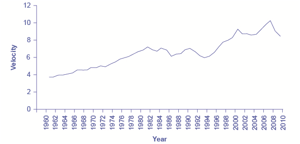
Velocity is the nominal GDP divided by the money supply for a given year. Different measures of velocity can be calculated by using different measures of the money supply. Velocity, as calculated by using M1, has lacked a steady trend since the 1980s, instead bouncing up and down. (credit: Federal Reserve Bank of St. Louis)
In the 1970s, when velocity as measured by M1 seemed predictable, a number of economists, led by Nobel laureate Milton Friedman (1912–2006), argued that the best monetary policy was for the central bank to increase the money supply at a constant growth rate. These economists argued that with the long and variable lags of monetary policy, and the political pressures on central bankers, central bank monetary policies were as likely to have undesirable as to have desirable effects. This led these economists to believe that the monetary policy should seek steady growth in the money supply of 3% per year. They argued that a steady rate of monetary growth would be correct over longer time periods, since it would roughly match the growth of the real economy. In addition, they argued that giving the central bank less discretion to conduct monetary policy would prevent an overly activist central bank from becoming a source of economic instability and uncertainty. In this spirit, Friedman wrote in 1967: “The first and most important lesson that history teaches about what monetary policy can do—and it is a lesson of the most profound importance—is that monetary policy can prevent money itself from being a major source of economic disturbance.”
As the velocity of M1 began to fluctuate in the 1980s, having the money supply grow at a predetermined and unchanging rate seemed less desirable, because as the quantity theory of money shows, the combination of constant growth in the money supply and fluctuating velocity would cause nominal GDP to rise and fall in unpredictable ways. The jumpiness of velocity in the 1980s caused many central banks to focus less on the rate at which the quantity of money in the economy was increasing, and instead to set monetary policy by reacting to whether the economy was experiencing or in danger of higher inflation or unemployment.
Unemployment and Inflation
If you were to survey central bankers around the world and ask them what they believe should be the primary task of monetary policy, the most popular answer by far would be fighting inflation. Most central bankers believe that the neoclassical model of economics accurately represents the economy over the medium to long term. Remember that in the neoclassical model of the economy, the aggregate supply curve is drawn as a vertical line at the level of potential GDP, as shown in Figure 10. In the neoclassical model, the level of potential GDP (and the natural rate of unemployment that exists when the economy is producing at potential GDP) is determined by real economic factors. If the original level of aggregate demand is AD0, then an expansionary monetary policy that shifts aggregate demand to AD1 only creates an inflationary increase in the price level, but it does not alter GDP or unemployment. From this perspective, all that monetary policy can do is to lead to low inflation or high inflation—and low inflation provides a better climate for a healthy and growing economy. After all, low inflation means that businesses making investments can focus on real economic issues, not on figuring out ways to protect themselves from the costs and risks of inflation. In this way, a consistent pattern of low inflation can contribute to long-term growth.
Velocity Calculated Using M1
Velocity is the nominal GDP divided by the money supply for a given year. Different measures of velocity can be calculated by using different measures of the money supply. Velocity, as calculated by using M1, has lacked a steady trend since the 1980s, instead bouncing up and down. (credit: Federal Reserve Bank of St. Louis)
In the 1970s, when velocity as measured by M1 seemed predictable, a number of economists, led by Nobel laureate Milton Friedman (1912–2006), argued that the best monetary policy was for the central bank to increase the money supply at a constant growth rate. These economists argued that with the long and variable lags of monetary policy, and the political pressures on central bankers, central bank monetary policies were as likely to have undesirable as to have desirable effects. This led these economists to believe that the monetary policy should seek steady growth in the money supply of 3% per year. They argued that a steady rate of monetary growth would be correct over longer time periods, since it would roughly match the growth of the real economy. In addition, they argued that giving the central bank less discretion to conduct monetary policy would prevent an overly activist central bank from becoming a source of economic instability and uncertainty. In this spirit, Friedman wrote in 1967: “The first and most important lesson that history teaches about what monetary policy can do—and it is a lesson of the most profound importance—is that monetary policy can prevent money itself from being a major source of economic disturbance.”
As the velocity of M1 began to fluctuate in the 1980s, having the money supply grow at a predetermined and unchanging rate seemed less desirable, because as the quantity theory of money shows, the combination of constant growth in the money supply and fluctuating velocity would cause nominal GDP to rise and fall in unpredictable ways. The jumpiness of velocity in the 1980s caused many central banks to focus less on the rate at which the quantity of money in the economy was increasing, and instead to set monetary policy by reacting to whether the economy was experiencing or in danger of higher inflation or unemployment.
Unemployment and Inflation
If you were to survey central bankers around the world and ask them what they believe should be the primary task of monetary policy, the most popular answer by far would be fighting inflation. Most central bankers believe that the neoclassical model of economics accurately represents the economy over the medium to long term. Remember that in the neoclassical model of the economy, the aggregate supply curve is drawn as a vertical line at the level of potential GDP, as shown in Figure 10. In the neoclassical model, the level of potential GDP (and the natural rate of unemployment that exists when the economy is producing at potential GDP) is determined by real economic factors. If the original level of aggregate demand is AD0, then an expansionary monetary policy that shifts aggregate demand to AD1 only creates an inflationary increase in the price level, but it does not alter GDP or unemployment. From this perspective, all that monetary policy can do is to lead to low inflation or high inflation—and low inflation provides a better climate for a healthy and growing economy. After all, low inflation means that businesses making investments can focus on real economic issues, not on figuring out ways to protect themselves from the costs and risks of inflation. In this way, a consistent pattern of low inflation can contribute to long-term growth.
Monetary Policy in a Neoclassical Model
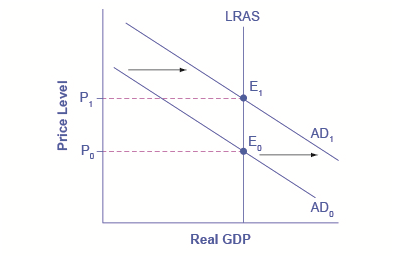
In a neoclassical view, monetary policy affects only the price level, not the level of output in the economy. For example, an expansionary monetary policy causes aggregate demand to shift from the original AD0 to AD1. However, the adjustment of the economy from the original equilibrium (E0) to the new equilibrium (E1) represents an inflationary increase in the price level from P0 to P1, but has no effect in the long run on output or the unemployment rate. In fact, no shift in AD will affect the equilibrium quantity of output in this model.
This vision of focusing monetary policy on a low rate of inflation is so attractive that many countries have rewritten their central banking laws since in the 1990s to have their bank practice inflation targeting, which means that the central bank is legally required to focus primarily on keeping inflation low. By 2010, central banks in 26 countries, including Austria, Brazil, Canada, Israel, Korea, Mexico, New Zealand, Spain, Sweden, Thailand, and the United Kingdom faced a legal requirement to target the inflation rate. A notable exception is the Federal Reserve in the United States, which does not practice inflation-targeting. Instead, the law governing the Federal Reserve requires it to take both unemployment and inflation into account.
Economists have no final consensus on whether a central bank should be required to focus only on inflation or should have greater discretion. For those who subscribe to the inflation targeting philosophy, the fear is that politicians who are worried about slow economic growth and unemployment will constantly pressure the central bank to conduct a loose monetary policy—even if the economy is already producing at potential GDP. In some countries, the central bank may lack the political power to resist such pressures, with the result of higher inflation, but no long-term reduction in unemployment. The U.S. Federal Reserve has a tradition of independence, but central banks in other countries may be under greater political pressure. For all of these reasons—long and variable lags, excess reserves, unstable velocity, and controversy over economic goals—monetary policy in the real world is often difficult. The basic message remains, however, that central banks can affect aggregate demand through the conduct of monetary policy and in that way influence macroeconomic outcomes.
Asset Bubbles and Leverage Cycles
One long-standing concern about having the central bank focus on inflation and unemployment is that it may be overlooking certain other economic problems that are coming in the future. For example, from 1994 to 2000 during what was known as the “dot-com” boom, the U.S. stock market, which is measured by the Dow Jones Industrial Index (which includes 30 very large companies from across the U.S. economy), nearly tripled in value. The Nasdaq Index, which includes many smaller technology companies, increased in value by a multiple of five from 1994 to 2000. These rates of increase were clearly not sustainable. Indeed, stock values as measured by the Dow Jones were almost 20% lower in 2009 than they had been in 2000. Stock values in the Nasdaq index were 50% lower in 2009 than they had been in 2000. The drop-off in stock market values contributed to the recession of 2001 and the higher unemployment that followed.
A similar story can be told about housing prices in the mid-2000s. During the 1970s, 1980s, and 1990s, housing prices increased at about 6% per year on average. During what came to be known as the “housing bubble” from 2003 to 2005, housing prices increased at almost double this annual rate. These rates of increase were clearly not sustainable. When the price of housing fell in 2007 and 2008, many banks and households found that their assets were worth less than they expected, which contributed to the recession that started in 2007.
At a broader level, some economists worry about a leverage cycle, where “leverage” is a term used by financial economists to mean “borrowing.” When economic times are good, banks and the financial sector are eager to lend, and people and firms are eager to borrow. Remember that the amount of money and credit in an economy is determined by a money multiplier—a process of loans being made, money being deposited, and more loans being made. In good economic times, this surge of lending exaggerates the episode of economic growth. It can even be part of what lead prices of certain assets—like stock prices or housing prices—to rise at unsustainably high annual rates. At some point, when economic times turn bad, banks and the financial sector become much less willing to lend, and credit becomes expensive or unavailable to many potential borrowers. The sharp reduction in credit, perhaps combined with the deflating prices of a dot-com stock price bubble or a housing bubble, makes the economic downturn worse than it would otherwise be.
Thus, some economists have suggested that the central bank should not only just look at economic growth, inflation, and unemployment rates, but should also keep an eye on asset prices and leverage cycles. Such proposals are quite controversial. If a central bank had announced in 1997 that stock prices were rising “too fast” or in 2004 that housing prices were rising “too fast,” and then taken action to hold down price increases, many people and their elected political representatives would have been outraged. Neither the Federal Reserve nor any other central banks want to take the responsibility of deciding when stock prices and housing prices are too high, too low, or just right. As further research explores how asset price bubbles and leverage cycles can affect an economy, central banks may need to think about whether they should conduct monetary policy in a way that would seek to moderate these effects.
Let’s end this section with how the Fed—or any central bank—would stir up the economy by increasing the money supply.
Calculating the Effects of Monetary Stimulus
Suppose that the central bank wants to stimulate the economy by increasing the money supply. The bankers estimate that the velocity of money is 3, and that the price level will increase from 100 to 110 due to the stimulus. Using the quantity equation of money, what will be the impact of an $800 billion dollar increase in the money supply on the quantity of goods and services in the economy given an initial money supply of $4 trillion?
Step 1. We begin by writing the quantity equation of money: MV = PQ. We know that initially V = 3, M = 4,000 (billion) and P = 100. Substituting these numbers in, we can solve for Q:
MV = PQ
4,000 × 3 = 100 × Q
Q = 120
Step 2. Now we want to find the effect of the addition $800 billion in the money supply, together with the increase in the price level. The new equation is:
MV= PQ
4,800 × 3 = 110 × Q
Q = 130.9
Step 3. If we take the difference between the two quantities, we find that the monetary stimulus increased the quantity of goods and services in the economy by 10.9 billion.
The discussion in this chapter has focused on domestic monetary policy; that is, the view of monetary policy within an economy.
The Problem of the Zero Percent Interest Rate Lower Bound
In 2008, the U.S. Federal Reserve found itself in a difficult position. The federal funds rate was on its way to near zero, which meant that traditional open market operations by which the Fed purchases U.S. Treasury Bills to lower short term interest rates, was no longer viable. This so called “zero bound problem,” prompted the Fed, under then Chair Ben Bernanke, to attempt some unconventional policies, collectively called quantitative easing. By early 2014, quantitative easing nearly quintupled the amount of bank reserves. This likely contributed to the U.S. economy’s recovery, but the impact was muted. This was probably due to some of the hurdles mentioned in the last section of this module. The unprecedented increase in bank reserves also led to fears of inflation. Whether or not the Fed will be able to suck this liquidity out of the system to avoid an inflationary boom as the economy recovers remain to be seen.
Monetary policy is inevitably imprecise, for a number of reasons: (a) the effects occur only after long and variable lags; (b) if banks decide to hold excess reserves, monetary policy cannot force them to lend; and (c) velocity may shift in unpredictable ways. The basic quantity equation of money is MV = PQ, where M is the money supply, V is the velocity of money, P is the price level, and Q is the real output of the economy. Some central banks, like the European Central Bank, practice inflation targeting, which means that the only goal of the central bank is to keep inflation within a low target range. Other central banks, such as the U.S. Federal Reserve, are free to focus on either reducing inflation or stimulating an economy that is in recession, whichever goal seems most important at the time.
Video: Finance Tips: Prime Interest Rate Tips
 Answer the self check questions below to monitor your understanding of the concepts in this section.
Self Check Questions
- What does the monetary policy impact in the short run? In the long run?
- How long does it take for the monetary policy to work?
- Define the term "prime rate."
- Research online the current interest rates for: (a) a small business loan, (b) a new car, (c) a used car, (d) a small personal loan, and (e) a mortgage for an existing home.
- What does it mean to "monetize the debt"? Why would the government do this?
- What should the Federal Reserve do if forced to choose between inflation or high interest rates?
- When the Federal Reserve conducts monetary policy, what are two things it cannot control? Explain.
- What is the impact on the economy of an easy money policy?
- What is the impact on the economy of a tight money policy?
- How do politics influence interest rates?