8.1.5: Tables to Find Limits

Tables to Find Limits

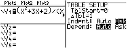
Calculators such as the TI-84 have a table view that allows you to make extremely educated guesses as to what the limit of a function will be at a specific point, even if the function is not actually defined at that point.

How could you use a table to calculate the following limit?

\(\ \lim _{x \rightarrow-1} \frac{x^{2}+3 x+2}{x+1}\)

---

Using Tables to Find Limits

If you were given the following information organized in a table, how would you fill in the center column?

3.9	3.99	3.999		4.001	4.01	4.1
12.25	12.01	12.00001		11.99999	11.99	11.75

It would be logical to see the symmetry and notice how the top row approaches the number 4 from the left and the right. It would also be logical to notice how the bottom row approaches the number 12 from the left and the right. This would lead you to the conclusion that the limit of the function represented by this table is 12 as the top row approaches 4. It would not matter if the value at 4 was undefined or defined to be another number like 17, the pattern tells you that the limit at 4 is 12.

Using tables to help evaluate limits numerically requires this type of logic. Numerically is a term used to describe one of several different representations in mathematics. It refers to tables where the actual numbers are visible.

To estimate the limit \(\ \lim _{x \rightarrow 2} \frac{x-2}{x^{2}-x-2}\), complete the table:

x	1.9	1.99	1.999	2.001	2.01	2.1
f(x)

While it is not necessary to use the table feature in the calculator, it is very efficient.

To use a table on your calculator to evaluate a limit:

1. Enter the function on the y=screen
2. Go to table set up and highlight “ask” for the independent variable
3. Go to the table and enter values close to the number that x approaches

Another option is to substitute the given \(\ x\) values into the expression \(\ \frac{x-2}{x^{2}-x-2}\) and record your results. Either way, the completed table is as follows.

x	1.9	1.99	1.999	2.001	2.01	2.1
f(x)	0.34483	0.33445	0.33344	0.33322	0.33223	0.32258

The evidence suggests that the limit is \(\ \frac{1}{3}\).

---

Examples

Example 1

Earlier, you were asked to find the limit of \(\ \lim _{x \rightarrow-1} \frac{x^{2}+3 x+2}{x+1}\).

Solution

When you enter values close to -1 in the table you get \(\ y\) values that are increasingly close to the number 1. This implies that the limit as \(\ x\) approaches -1 is 1. Notice that when you evaluate the function at -1, the calculator produces an error. This should lead you to the conclusion that while the function is not defined at \(\ x=−1\), the limit does exist.

Example 2

Complete the table and use the result to estimate the limit.

\(\ \lim _{x \rightarrow 2} \frac{x-2}{x^{2}-4}\)

x	1.9	1.99	1.999	2.001	2.01	2.1
f(x)

Solution

You can trick the calculator into giving a very exact answer by typing in 1.999999999999 because then the calculator rounds instead of producing an error.

x	1.9	1.99	1.999	2.001	2.01	2.1
f(x)	0.25641	0.25063	0.25006	0.24994	0.24938	0.2439

The evidence suggests that the limit is \(\ \frac{1}{4}\).

Example 3

Complete the table and use the result to estimate the limit.

\(\ \lim _{x \rightarrow 0} \frac{\sqrt{x+3}-\sqrt{3}}{x}\)

x	-0.1	-0.01	-0.001	0.001	0.01	0.1
f(x)

Solution

x	-0.1	-0.01	-0.001	0.001	0.01	0.1
f(x)	0.29112	0.28892	0.2887	0.28865	0.28843	0.28631

The evidence suggests that the limit is a number between 0.2887 and 0.28865. When you learn to find the limit analytically, you will know that the exact limit is \(\ \frac{1}{2} \cdot 3 \frac{1}{2} \approx 0.2886751346\).

Example 4

Graph the following function and the use a table to verify the limit as \(\ x\) approaches 1.

\(\ f(x)=\frac{x^{3}-1}{x-1}, x \neq 1\)

Solution

\(\ \lim _{x \rightarrow 1} f(x)=3\). This is because when you factor the numerator and cancel common factors, the function becomes a quadratic with a hole at the point \(\ (1, 3)\).

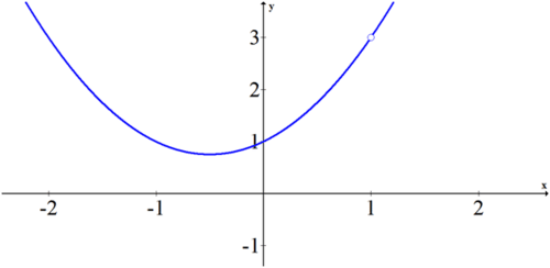
You can verify the limit in the table.

x	f(x)
.75	2.3125
.9	2.71
.99	2.9701
.999	2.997
1	Error
1.001	3.003
1.01	3.0301
1.1	3.31
1.25	3.8125

Example 5

Estimate the limit numerically.

\(\ \lim _{x \rightarrow 0} \frac{\left[\frac{4}{x+2}\right]-2}{x}\)

Solution

x	-0.1	-0.01	-0.001	0.001	0.01	0.1
f(x)	0.20526	0.02005	0.002	-0.002	-0.02	-0.1952

\(\ \lim _{x \rightarrow 0} f(x)=0\)

---

Review

Estimate the following limits numerically.

1. \(\ \lim _{x \rightarrow 5} \frac{x^{2}-25}{x-5}\)
2. \(\ \lim _{x \rightarrow-1} \frac{x^{2}-3 x-4}{x+1}\)
3. \(\ \lim _{x \rightarrow 2} \frac{x^{3}-5 x^{2}+2 x-4}{x^{2}-3 x+2}\)
4. \(\ \lim _{x \rightarrow 0} \frac{\sqrt{x+2}-\sqrt{2}}{x}\)
5. \(\ \lim _{x \rightarrow 3}\left(\frac{1}{x-3}-\frac{9}{x^{2}-9}\right)\)
6. \(\ \lim _{x \rightarrow 2} \frac{x^{2}+5 x-14}{x-2}\)
7. \(\ \lim _{x \rightarrow 1} \frac{x^{2}-8 x+7}{x-1}\)
8. \(\ \lim _{x \rightarrow 0} \frac{\sqrt{x+5}-\sqrt{5}}{x}\)
9. \(\ \lim _{x \rightarrow 9} \frac{\sqrt{x}-3}{x-9}\)
10. \(\ \lim _{x \rightarrow 0} \frac{x^{2}+5 x}{x}\)
11. \(\ \lim _{x \rightarrow-3} \frac{x^{2}-9}{x+3}\)
12. \(\ \lim _{x \rightarrow 4} \frac{\sqrt{x}-2}{x-4}\)
13. \(\ \lim _{x \rightarrow 2} \frac{\sqrt{x+3}-2}{x-1}\)
14. \(\ \lim _{x \rightarrow 5} \frac{x^{2}-25}{x^{3}-125}\)
15. \(\ \lim _{x \rightarrow-1} \frac{x-2}{x+1}\)

---

Review (Answers)

To see the Review answers, open this PDF file and look for section 14.3.

---

Vocabulary

Term	Definition
limit	A limit is the value that the output of a function approaches as the input of the function approaches a given value.
numerically	Numerically is a term used to describe one of several different representations in mathematics. It refers to tables where the actual numbers are visible.

---

Image Attributions

1. [Figure 1]
   Credit: CK-12 Foundation
   License: CC BY-SA