2.6.4: Intermediate Value Theorem

Intermediate Value Theorem

This lesson introduces two theorems: The Intermediate Value Theorem, and The Bounds on Zeros Theorem. A technical definition is given below, but what do these theorems really mean in 'ordinary language'?

---

Intermediate Value Theorem

The intermediate value theorem offers one way to find roots of a continuous function. An informal definition of continuous is that a function is continuous over a certain interval if it has no breaks, jumps, asymptotes, or holes in that interval. Polynomial functions are continuous for all real numbers x. Rational functions are often not continuous over the set of real numbers because of asymptotes or holes in the graph, but for intervals without holes, rational functions are continuous.

If we know a function is continuous over some interval [a,b], then we can use the intermediate value theorem:

If f(x) is continuous on some interval [a,b] and n is between f(a) and f(b), then there is some c∈[a,b] such that f(c)=n.

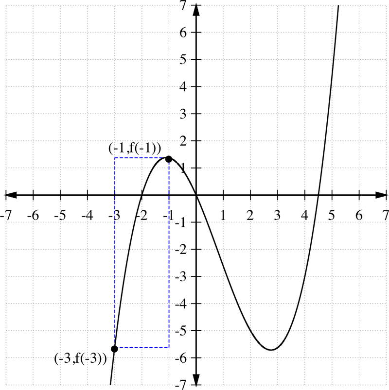
The following graphs highlight how the intermediate value theorem works. Consider the graph of the function \(\ f(x)=\frac{1}{4}\left(x^{3}-\frac{5 x^{2}}{2}-9 x\right)\) below on the interval [-3, -1].

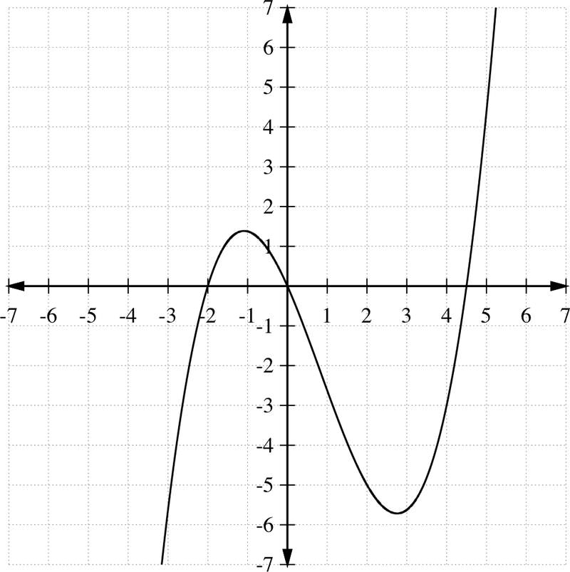
f(−3)=−5.625 and f(−1)=1.375. If we draw bounds on [-3, -1] and [f(−3), f(−1)], then we see that for any y−value between y=−5.625 and y=1.375, there must be an x value in [-3, -1] such that f(x)=y.

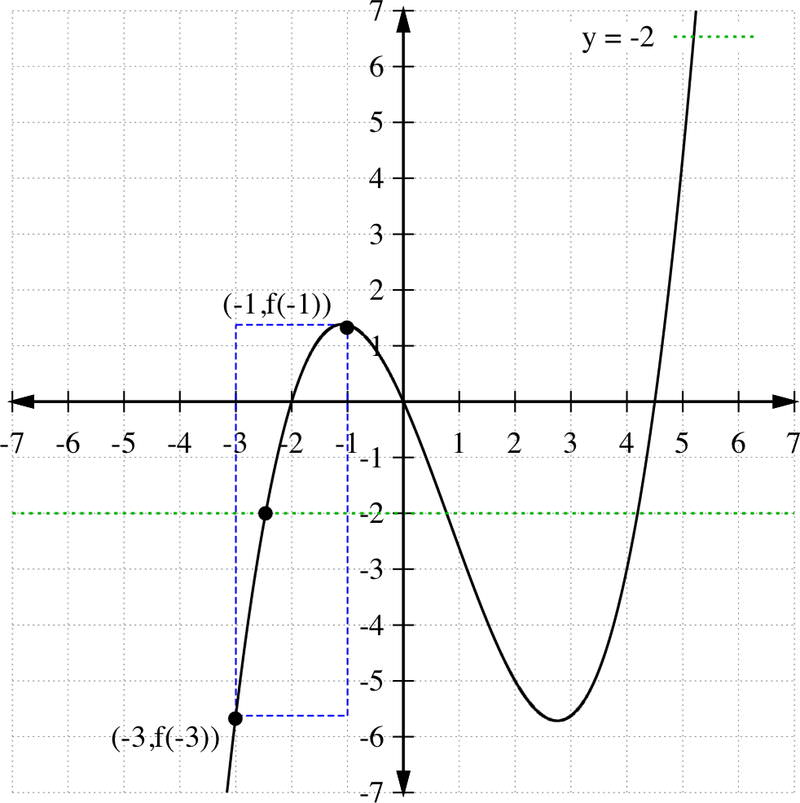
So, for example, if we choose c=−2, we know that for some x ∈ [−3,−1], f(x)=−2, even though solving this by hand would be a chore!

The Bounds on Zeros Theorem is a corollary to the Intermediate Value Theorem:

Bounds on Zeros Theorem

If f is continuous on [a,b] and there is a sign change between f(a) and f(b) (that is, f(a) is positive and f(b) is negative, or vice versa), then there is a c∈(a,b) such that f(c)=0.

The bounds on zeros theorem is a corollary to the intermediate value theorem because it is not fundamentally different from the general statement of the intermediate value theorem, just a special case where n=0.

Looking back at \(\ f(x)=\frac{1}{4}\left(x^{3}-\frac{5 x^{2}}{2}-9 x\right)\) above, because f(−3)<0 and f(−1)>0, we know that for some x∈[−3,−1], f(x) has a root. In fact, that root is at x=−2. and we can test that using synthetic division or by evaluating f(−2) directly.

Approximate Zeros of Polynomial Functions

In calculus you will learn several methods for numerically approximating the roots of functions. In this section we show one elementary numerical method for finding the zeros of a polynomial which takes advantage of the Intermediate Value Theorem.

Given a continuous function g(x),

1. Find two points such that g(a) > 0 and g(b) < 0. Once you have found these two points, you can iteratively use the steps below to find the root of g(x) on the interval [a,b]. (Note, we will assume a < b, but the same algorithm works with minor adjustments if b > a)
2. Evaluate \(\ g\left(\frac{a+b}{2}\right)\).
   1. If \(\ g\left(\frac{a+b}{2}\right)=0\), then the root is \(\ x=\frac{a+b}{2}\).
   2. If \(\ g\left(\frac{a+b}{2}\right)>0\), replace a with \(\ \frac{a+b}{2}\). and repeat steps 1-2 using \(\ \left[\frac{a+b}{2}, b\right]\)
   3. If \(\ g\left(\frac{a+b}{2}\right)<0\), replace b with \(\ \frac{a+b}{2}\). and repeat steps 1-2 using \(\ \left[a, \frac{a+b}{2}\right]\)

This algorithm will not usually find the exact root of g(x), but it will allow you to find a reasonably small interval for the root. For example, you could repeat this process enough times so that you find an interval with |a−b|<0.01, and you will know the root of g(x) within a reasonably good approximation. The quality of the approximation you use (and the number of steps you use) will depend on why you are looking for the root. For most applications coming within 0.01 of the root is a reasonable approximation, but for some applications (such as building a bridge or launching a rocket) you need much more accuracy.

An Interesting Corollary of the Intermediate Value Theorem

One surprising result of the Intermediate Value Theorem is that if you draw any great circle around the globe, then there must two antipodal points on that great circle that have exactly the same temperature.

Recall that a great circle is a path around a sphere that gives the shortest distance between any two points on the sphere. The equator is a great circle around the globe. Antipodal points are two points on opposite sides of the sphere. In the diagram below, B and B′ are antipodal.

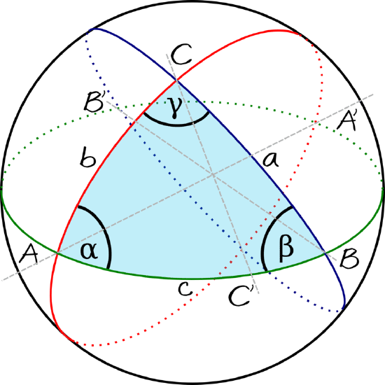
For an informal proof of this result, look at the image of a sphere with three great circles above. Suppose that the temperature at B is 75∘ and the temperature B′ is 50∘. The difference between the temperature at B and at B′ is 75−50=25. Now imagine rotating the segment \(\ \overline{B B^{\prime}}\) around the blue great circle. When the segment has rotated 180 degrees (i.e. when B has rotated to where B′ is), then the difference between the temperatures at these two points is 50−75=−25. Since temperatures vary continuously, by the intermediate value theorem, there must be some point on that circle when the difference was 0, implying two antipodal points had the same temperature.

Notice that this little demonstration does not tell us which two antipodal points had the same temperature, only that there must be two such points on any great circle.

---

Examples

Example 1

Earlier, you were asked if you could write less formal definitions of the Intermediate Value Theorem and the Bounds on Zeros Theorem.

Solution

One possibility might be:

The Intermediate Value Theorem simply states that if you know two points on a graph, and know that the graph includes all the points between them, then any point between them must be on the graph.

The Bounds on Zeros Theorem suggests that if a graph contains all of the points between a positive and a negative value, then a zero point between those two values is on the graph.

Example 2

Show that f(x)=−3x³+5x has at least one root in the interval [1, 2].

Solution

Since f(x) is a polynomial we know that it is continuous. f(1) = 2 and f(2) = −14. Let n = 0 ∈ [−14,2]. Applying the Intermediate Value Theorem, there must exist some point c ∈ [1,2] such that f(c) = 0. This proves that f(x) has a root in [1, 2].

Example 3

The table below shows several sample values of a polynomial p(x).

x	−4	−2	0	1	4	6	8	10	15	18
p(x)	44.15	6.62	−4.12	−4.09	1.16	0	−8.74	−24.07	−49.8918	3.41

Solution

Based on the information in the table:

a. What is the minimum number of roots of p(x)?

b. What are bounds on the roots of p(x) that you identified in (a)?

Since p(x) is a polynomial we already know that it is continuous. We can use the Intermediate Value Theorem to identify roots by looking at when p(x) changes from negative to positive, or from positive to negative.

a. There are four sign changes of p(x) in the table, so at minimum, p(x) has four roots.

b. The roots are in the following intervals x ∈ [−2, 0], x ∈ [1, 4], x ∈ [15, 18], and the table also tells us that one root is at x=6.

Example 4

Show the first 5 iterations of finding the root of h(x)=x²−x−1 using the starting values a=0 and b=2.

Solution

1. First we verify that there is a root between x=0 and x=2. h(0)=−1 and h(2)=1 so we know there is a root in the interval [0, 2]. Check \(\ h\left(\frac{2+0}{2}\right)=h(1)=-1\). Since −1 < 0 we know the root is between x=1 and x=2, and we use the new interval [1, 2].
2. Now we use the interval [1, 2]. \(\ h\left(\frac{1+2}{2}\right)=h(1.5)=-0.25\). Since −0.25 < 0, we use the interval [1.5, 2].
3. \(\ h\left(\frac{1.5+2}{2}\right)=h(1.75)=0.31\). Since 0.31 > 0, we know that the zero is in the interval [1.5, 1.75].
4. \(\ h\left(\frac{1.5+1.75}{2}\right)=h(1.625)=0.02\). Since 0.02 > 0, we know the root is between 1.5 and 1.625.
5. \(\ h\left(\frac{1.5+1.625}{2}\right)=h(1.5620)=-0.12\). Since −0.12 < 0, we know the root is between 1.5620 and 1.625.

This example shows that after five iterations we have narrowed the possible location of the root to within 0.06 units. Not bad!

Example 5

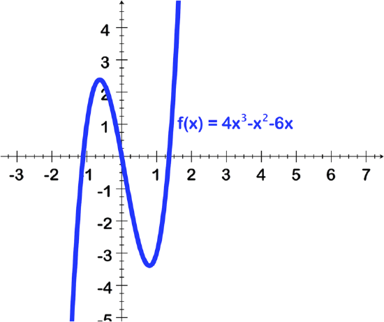
Use the image of the graph below to find the following:

1. Degree of the polynomial
2. Number of real zeros and their approximate values using the graph
3. Number of imaginary zeros

Solution

1. To identify the degree, recall that the degree of a polynomial is one number greater than the number of turns. The image shows turns at apx x = -.6 and apx x = .75, therefore this is a 3rd degree function.
2. The image shows the line crossing the x axis 3 times, at (apx) -1.15, at 0 and at (apx) 1.4.
3. Since this is a 3rd degree equation there are 3 possible zeros, and since there are 3 real zeros there are no imaginary ones.

Example 6

Show that f(x)=8x³−5x²−7x−5 has at least one root in the interval [1, 2].

Solution

Since f(x) is a polynomial we know that it is continuous. f(1) = −9 and f(2) = 25. Let n = 0 ∈ [−9, 25]. Applying the Intermediate Value Theorem, there must exist some point c ∈ [1,2] such that f(c) = 0. This proves that f(x) has a root in [1, 2].

Note that since this is a 3rd degree polynomial, there are three zeros. Since there is only one real zero, the other two must be imaginary.

---

Review

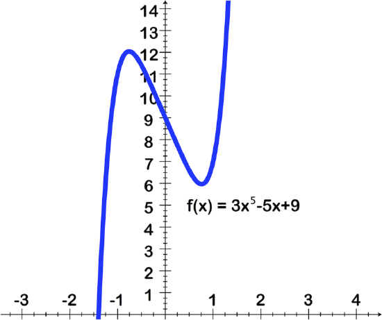
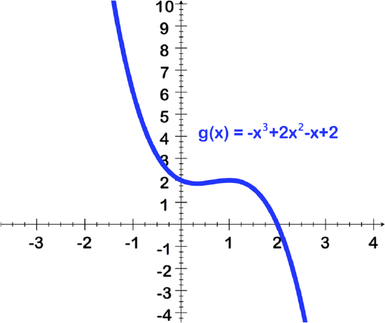
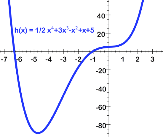
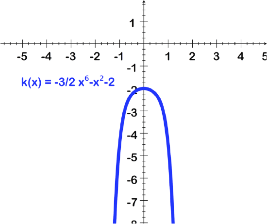
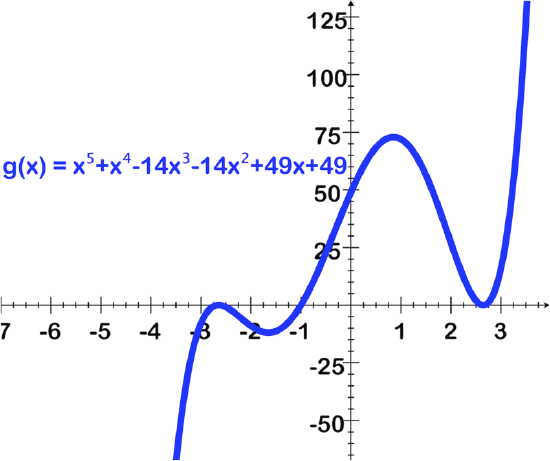
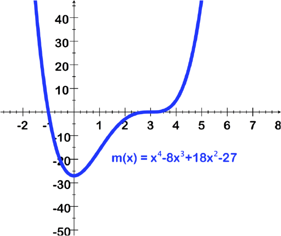
For questions 1 - 6, use the image of the graph to find the following:

1. Leading coefficient and degree of the polynomial
2. Number of real zeros and their approximate values using the graph
3. Number of imaginary zeros

[Figure1]

2.

[Figure2]

3.

[Figure3]

4.

5.

[Figure4]

6.

[Figure5]

For questions 7-12, use the intermediate value theorem to show the bounds on the zeros of each function. (Your bounds should be within the whole number)

7. f(x)=2x³−3x+4
8. g(x)=−5x²+8x+12
9. \(\ h(x)=\frac{1}{2} x^{4}-x^{3}-3 x^{2}+1\)
10. \(\ j(x)=-\frac{2}{x^{2}+1}+\frac{1}{2}\)
11. k(x) is a polynomial and selected values of k(x) are given in the following table:

    x	-3	-2	-1	0	1	2	3
    k(x)	−23.5	−1	0.5	−1	.5	−1	−23.5

12. Stephen argues the function \(\ r(x)=\frac{4 x+1}{x+3.5}\) has two zeros based on the following table and an application of the Bounds on Zeros Theorem. What is faulty about Stephen's reasoning?

    x	−5	−4	−3	−2	−1	0	1	2	3	4
    r(x)	12.67	30	−22	−4.67	-1.20	0.29	1.11	1.64	2.0	2.27

For questions 13-15, apply the numerical algorithm five times to find a bound on the zeros of the following functions given the indicated starting values. Give a final estimate for the zero.

13. k(x)=x⁴−3x+1 on [0,1]
14. b(x)=−0.1x⁵+3x³−5x² on [1,3]
15. \(\ c(x)=\frac{3 x^{2}-2}{x^{4}+2} \text { on }[0,2]\)

---

Review (Answers)

To see the Review answers, open this PDF file and look for section 2.13.

---

Vocabulary

Term	Definition
Bounds on Zeros Theorem	The bounds on zeros theorem states that if f is continuous on [a,b] and there is a sign change between f(a) and f(b) (that is, f(a) is positive and f(b) is negative, or vice versa), then there is a c ∈ (a, b) such that f(c) = 0.
Continuous	Continuity for a point exists when the left and right sided limits match the function evaluated at that point. For a function to be continuous, the function must be continuous at every single point in an unbroken domain.
Continuous Function	A continuous function is a function without breaks or gaps. It contains an infinite, uncountable number of values.
intermediate value theorem	The intermediate value theorem states that if f(x) is continuous on some interval [a, b] and n is between f(a) and f(b), then there is some c ∈ [a, b] such that f(c) = n.
interval	An interval is a specific and limited part of a function.
Rational Function	A rational function is any function that can be written as the ratio of two polynomial functions.
Synthetic Division	Synthetic division is a shorthand version of polynomial long division where only the coefficients of the polynomial are used.
theorem	A theorem is a statement that can be proven true using postulates, definitions, and other theorems that have already been proven.
Zeroes	The zeroes of a function f(x) are the values of x that cause f(x) to be equal to zero.
Zeros	The zeros of a function f(x) are the values of x that cause f(x) to be equal to zero.

---

Image Attributions

1. [Figure 1]
   Credit: CK-12
   Source: CK-12
2. [Figure 2]
   Credit: CK-12
   Source: CK-12
3. [Figure 3]
   Credit: CK-12
   Source: CK-12
4. [Figure 4]
   Credit: CK-12
   Source: CK-12
5. [Figure 5]
   Credit: CK-12
   Source: CK-12