7.1: Derivatives with Mean Value Theorem and Rolle's Theorem
- Page ID
- 1213
Jim was telling his math major friend about a speeding ticket he had received recently for going over 80 mph one weekend morning when there was little traffic on the highway. Apparently two police officers at different locations along the highway had recorded him going 60 and 65 mph respectively as he went by each of their speed trap positions. Jim said he knew where the speed traps were located and always made sure he was within the speed limit going by, so he could not understand how they could say he was speeding. Jim’s math major friend asked whether the officer who issued the ticket had said anything. Jim recalled that the officer had mentioned that the speed traps were exactly 3 miles apart, and that they knew Jim’s car had covered the distance in 2 minutes. Jim’s math major friend smiled and said, “Oh, that’s how they did it: The Mean Value Theorem”. Jim looked very perplexed.
Can you figure out how the police officer could have issued a ticket without actually witnessing Jim’s car going over 80 mph?
The Mean Value Theorem
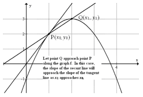
In an earlier concept, the derivative of a function was introduced as the slope of the tangent line at a point. We looked at how the slope of a secant line changed as one of the two points approached the other. The secant line became the tangent line in the limit as illustrated below.

CC BY-NC-SA
Now we look at the slope values of tangent lines in an interval defined by the secant line between two points. The following theorem gives an important relationship.
Rolle’s Theorem: If f is continuous on a closed interval [a,b] and differentiable on the open interval (a,b), and if f(a)=f(b) then f has at least one value c in the open interval (a,b) such that f′(c)=0.
Let’s see if you can make use of Rolle’sTheorem
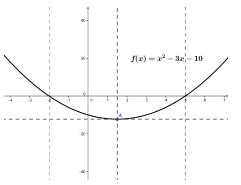
For the function \( f(x)=x^2−3x−10 \nonumber\), show that it satisfies the conditions of Rolle’s theorem on the interval [-2, 5] and find all numbers c in (-2, 5) that satisfy f′(c)=0

CC BY-NC-SA
Evaluating f(x) at x=−2 and x=5 yields:
\[ f(−2)=(−2)^2−3(−2)−10 \nonumber\]
\[ =0 \nonumber\]
\[ f(5)=(5)^2−3(5)−10 \nonumber\]
\[ =0 \nonumber\]
Therefore f(−2)=f(5), which satisfies the conditions for Rolle’s theorem to hold.
Now to find values of c that satisfy f′(c)=0.
\[ \frac{dy}{dx} =2x−3 \nonumber\]
\[ f′(c)=0 \nonumber\]
\[ =2(c)−3 \nonumber\]
\[ ∴c= \frac{3}{2} \nonumber\]
So \( f′( \frac{3}{2})=0 \nonumber\) satisfies Rolle’sTheorem.
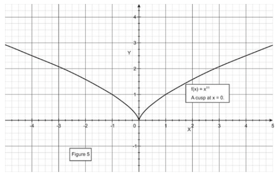
Consider the function \( f(x)=x^{ \frac{2}{3}} \nonumber\). On the interval [-4, 4], f(−4)=f(4). However, is there any point at which the derivative of \( f(x)=x^{ \frac{2}{3}} \nonumber\) is equal to zero? Is this a contradiction of Rolle's theorem?
The function curve for \( f(x)=x^{ \frac{2}{3}} \nonumber\) is shown below.

CC BY-NC-SA
It’s derivative is \( f′(x)= \frac{2}{3x^{ \frac{1}{3}}} \nonumber\), which is undefined at x=0, and there is no point at which the derivative is 0. But, because the function is not differentiable over the interval, Rolle’sTheorem does not apply. There is no contradiction.
Rolle’s Theorem requires that f(a)=f(b). But Rolle’s theorem is the basis for proving the important general theorem called the Mean Value Theorem which does not require f(a)=f(b).
Mean Value Theorem: If f is a continuous function on a closed interval [a,b] and if f′ contains the open interval (a,b) in its domain, then there exists a number c in the interval (a,b) such that
\[ f′(c)= \frac{f(b)−f(a)}{b−a} \nonumber\]
An equivalent form is: \( f(b)−f(a)=(b−a)f′(c) \nonumber\).
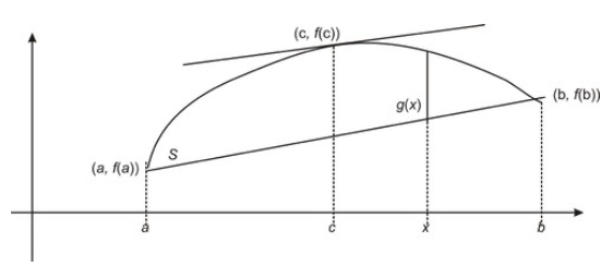
An illustration of the meaning of the Mean Value Theorem is shown in the figure below, where the slope of the secant line connecting f(a) and f(b) can be found to be the same as the slope of the tangent line at f(c).

CC BY-NC-SA
Verify that the Mean Value Theorem applies for the function \( f(x)=x^3+3x^2−24x \nonumber\) on the interval [1, 4].
We need to find c in the interval (1, 4) such that \( f′(c)= \frac{f(4)−f(1)}{(4−1)} \nonumber\)
\[ f′(c)= \frac{f(4)−f(1)}{(4−1)} \nonumber\]
\[ =16+203 \nonumber\]
\[ =12 \nonumber\]
Note that
\[ f′(x)=3x^2+6x−24 \nonumber\]
Hence, we must solve the following equation:
\[ 3c^2+6c−24=12 \nonumber\]
\[ 3c^2+6c−32=0 \nonumber\]
\[ c^2+2c−12=0 \nonumber\]
\[ c=−1± \sqrt{13} \nonumber\]
Since we need to have c in the interval (1, 4), the positive root is the solution:
c≈2.61.
Examples
Example 1
Earlier, you were asked about how Jim could get a speeding ticket for going at least 80 mph when his car’s speed was recorded at 60 mph and 65 mph.
The key information was that the police officer determined that Jim had traveled 3 miles in 2 minutes, so that Jim’s average speed was 90 mph. Jim’s math major friend knew that by the Mean Value Theorem there had to have been at least one time when Jim’s actual speed was 90 mph, definitely exceeding 80 mph.
Example 2
Verify that the Mean Value Theorem applies for the function \( f(x)=2sinx+3cosx \nonumber\) on the interval \( (0,2π) \nonumber\).
We need to find c in the interval (0,2π) such that \( f′(c)= \frac{f(2π)−f(0)}{(2π−0)} \nonumber\):
\[ f′(c)= \frac{f(2π)−f(0)}{(2π−0)} \nonumber\]
\[ = \frac{2−2}{2π} \nonumber\]
\[ =0 \nonumber\]
Note that
\[ f′(x)=2cosx−3sinx \nonumber\]
Hence, we must solve the following equation:
\[ 2cosc−3sinc=0 \nonumber\]
\[ tanc= \frac{2}{3} \nonumber\]
\[ c=tan^{−1} ( \frac{2}{3}) \nonumber\]
\( c=0.588 \nonumber\) radians … and also \( (0.588+π) \nonumber\) radians in the interval \( (0,2π) \nonumber\).
The Mean Value Theorem applies in two places in the interval \( (0,2π) \nonumber\).
Review
For #1-5, if possible, verify Rolle’s Theorem for the following functions by finding values of x for which f(x)=0 and f′(x)=0. If it is not possible, state why.
- \( f(x)=3x^3−12x \nonumber\)
- \( f(x)=x^2−2x−1 \nonumber\)
- \( f(x)=−2x^2−12x+5 \nonumber\)
- \( f(x)=|2x−3| \nonumber\)
- \( f(x)=2sinx+3cosx \nonumber\)
- \( f(x)=x^4−2x^2 \nonumber\)
- Prove that if the equation \( x^3+a_1x^2+a_2x=0 \nonumber\) has a positive root at x=r and that the equation \( 3x^2+2a_1x+a_2=0 \nonumber\) has a positive root less than r.
For #8-15, verify that the Mean Value Theorem works for each function in the specified interval, or state why it does not.
- \( f(x)=(x+2)x, [1, 2] \nonumber\)
- \( f(x)=2x, [-1,1] \nonumber\)
- \( f(x)=x^2−5x+1, [0, 3] \nonumber\)
- \( f(x)=5−4x, [1, 4] \nonumber\)
- \( f(x)=x^3−8x−5, [1, 4] \nonumber\)
- \( f(x)=sinx, [0, \frac{π}{2}] \nonumber\)
- \( f(x)=cosx, [0, \frac{π}{2}] \nonumber\)
- \( f(x)=2x, [0, 3] \nonumber\)
Vocabulary
| Term | Definition |
|---|---|
| mean value theorem | The mean value theorem for definite integrals states that if f is continuous on the closed interval [a,b] then at some point c in the open interval (a,b): \( \int\limits_{a}^{b} f(x)dx=f(c)(b−a) \nonumber\) |
| Rolle's theorem | Rolle’s theorem says that a function that has the same value at two points has a derivative of 0 at at least one point in the interval |
Additional Resources
PLIX: Play, Learn, Interact, eXplore - Maxima and Minima, Mean Value Theorem, Rolle's Theorem
Video: Mean Value Theorem
Practice: Derivatives with Mean Value Theorem and Rolle's Theorem
Real World: Droning On

