
5.2: Standard Deviation of a Data Set
- Page ID
- 5726
Standard Deviation of a Data Set
In a previous concept, you learned that standard deviation is a measure of the spread of a set of data away from the mean of the data.
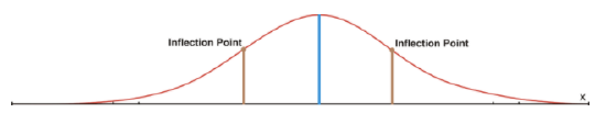
In a normal distribution, on either side of the line of symmetry, the curve appears to change its shape from being concave down (looking like an upside-down bowl) to being concave up (looking like a right-side-up bowl). Where this happens is called an inflection point of the curve. If a vertical line is drawn from an inflection point to the x-axis, the difference between where the line of symmetry goes through the x-axis and where this line goes through the x-axis represents 1 standard deviation away from the mean. Approximately 68% of all the data is located within 1 standard deviation of the mean.
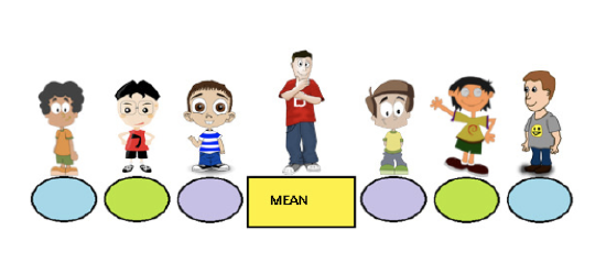
To emphasize this fact and the fact that the mean is the middle of the distribution, let’s play a game of Simon Says. Using color paper and 2 types of shapes, arrange the pattern of the shapes on the floor as shown below. Randomly select 7 students from your class to play the game. You will be Simon, and you are to give orders to the selected students. Only when Simon Says are the students to obey the given order. The orders can be given in many ways, but 1 suggestion is to deliver the following orders:
- “Simon Says for Frank to stand on the rectangle.”
- “Simon Says for Joey to stand on the closest oval to the right of Frank.”
- “Simon Says for Liam to stand on the closest oval to the left of Frank.”
- “Simon Says for Mark to stand on the farthest oval to the right of Frank.”
- “Simon Says for Juan to stand on the farthest oval to the left of Frank.”
- “Simon Says for Jacob to stand on the middle oval to the right of Frank.”
- “Simon Says for Sean to stand on the middle oval to the left of Frank.”
Once the students are standing in the correct places, pose questions about their positions with respect to Frank. The members of the class who are not playing the game should be asked to respond to these questions about the position of their classmates. Some questions that should be asked are the following:
- “Which 2 students are standing closest to Frank?”
- “Are Joey and Liam both the same distance away from Frank?”
- “Which 2 students are furthest away from Frank?”
- “Are Mark and Juan both the same distance away from Frank?”
When the students have completed playing Simon Says, they should have an understanding of the concept that the mean is the middle of the distribution and the remainder of the distribution is evenly spread out on either side of the mean.
The picture below is a simplified form of the game you have just played. The yellow rectangle is the mean, and the remaining rectangles represent 3 steps to the right of the mean and 3 steps to the left of the mean.
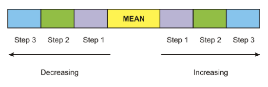
If we consider the spread of the data away from the mean, which is measured using standard deviation, as being a stepping process, then 1 step to the right or 1 step to the left is considered 1 standard deviation away from the mean. 2 steps to the left or 2 steps to the right are considered 2 standard deviations away from the mean. Likewise, 3 steps to the left or 3 steps to the right are considered 3 standard deviations away from the mean. The standard deviation of a data set is simply a value, and in relation to the stepping process, this value would represent the size of your footstep as you move away from the mean. Once the value of the standard deviation has been calculated, it is added to the mean for moving to the right and subtracted from the mean for moving to the left. If the value of the yellow mean tile was 58, and the value of the standard deviation was 5, then you could put the resulting sums and differences on the appropriate tiles.
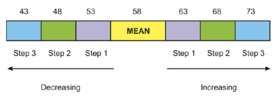
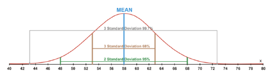
For a normal distribution, 68% of the data values would be located within 1 standard deviation of the mean, which is between 53 and 63. Also, 95% of the data values would be located within 2 standard deviations of the mean, which is between 48 and 68. Finally, 99.7% of the data values would be located within 3 standard deviations of the mean, which is between 43 and 73. The percentages mentioned here make up what statisticians refer to as the 68-95-99.7 Rule. These percentages remain the same for all data that can be assumed to be normally distributed. The following diagram represents the location of these values on a normal distribution curve.
Now that you understand the distribution of the data and exactly how it moves away from the mean, you are ready to calculate the standard deviation of a data set. For the calculation steps to be organized, a table is used to record the results for each step. The table will consist of 3 columns. The first column will contain the data and will be labeled x. The second column will contain the differences between the data values and the mean of the data set. This column will be labeled (x−x̅) for a sample and (x−μ) for a population. The final column will be labeled (x−x̅)2 for a sample and (x−μ)2 for a population, and it will contain the square of each of the values recorded in the second column.
If we were to add the variations found in the second column of the table, the total would be 0. This result of 0 implies that there is no variation between the data value and the mean. In other words, if we were conducting a survey of the number of hours that students use a cell phone in 1 day, and we relied upon the sum of the variations to give us some pertinent information, the only thing that we would learn is that all the students who participated in the survey use a cell phone for the exact same number of hours each day. We know that this is not true, because the survey does not show all the responses as being the same. In order to ensure that these variations do not lose their significance when added, the variation values are squared prior to calculating their sum.
What we need for a normal distribution is a measure of spread that is proportional to the scatter of the data, independent of the number of values in the data set and independent of the mean. The spread will be small when the data values are consistent, but large when the data values are inconsistent. The reason that the measure of spread should be independent of the mean is because we are not interested in this measure of central tendency, but rather, only in the spread of the data. For a normal distribution, the standard deviation fits the above profile for an appropriate measure of spread, and this value can be calculated for the set of data.
The standard deviation of a data set is always a positive value.
Calculating the Standard Deviation
1. A company wants to test its exterior house paint to determine how long it will retain its original color before fading. The company mixes 2 brands of paint by adding different chemicals to each brand. 6 one-gallon cans are made for each paint brand, and the results are recorded for every gallon of each brand of paint. The following are the results obtained in the laboratory:
| Brand A (Time in months) | Brand B (Time in months) |
|---|---|
| 15 | 40 |
| 65 | 50 |
| 55 | 35 |
| 35 | 40 |
| 45 | 45 |
| 25 | 30 |
Calculate the standard deviation for each brand of paint. Which brand has more variable data? These are both small populations.
| x | (x−μ) | (x−μ)2 |
|---|---|---|
| 15 | −25 | 625 |
| 65 | 25 | 625 |
| 55 | 15 | 225 |
| 35 | −5 | 25 |
| 45 | 5 | 25 |
| 25 | −15 | 225 |
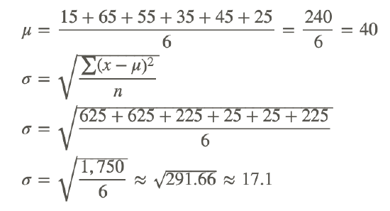
The standard deviation for Brand A is approximately 17.1.
| x | (x−μ) | (x−μ)2 |
|---|---|---|
| 40 | 0 | 0 |
| 50 | 10 | 100 |
| 35 | −5 | 25 |
| 40 | 0 | 0 |
| 45 | 5 | 25 |
| 30 | −10 | 100 |
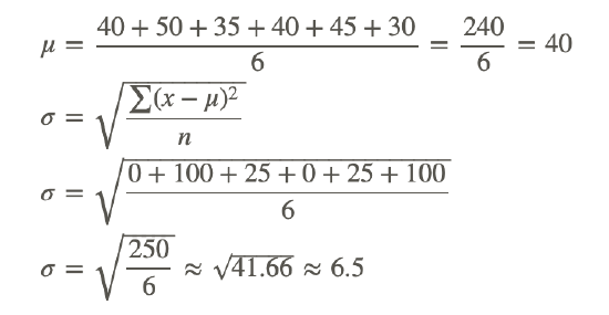
The standard deviation for Brand B is approximately 6.5.
The standard deviation for Brand A (17.1) was much larger than that for Brand B (6.5). However, the means of both brands were the same. When the means are equal, the larger the standard deviation is, the more variable are the data. Therefore, Brand A had more variable data.
2. Suppose the data for the 2 brands of paint in Example A represented samples instead of small populations. What would be the standard deviation of the data for the 2 brands?
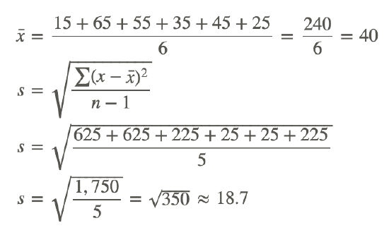
When calculating the standard deviation of a sample, it's necessary to divide by 1 less than the number of data values instead of by the number of data values. With this in mind, let's first calculate the standard deviation of the data for Brand A had it been a sample:
Now let's calculate the standard deviation of the data for Brand B had it been a sample:
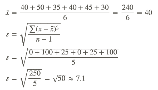
Notice that the standard deviation of the data for Brand A (18.7) is still much larger than the standard deviation of the data for Brand B (7.1).
Understanding Proportions of Data
Suppose data are normally distributed, with a mean of 84 and a standard deviation of 18. Between what 2 values will the following proportions of the data fall?
a. 68%
68% of the data will fall within 1 standard deviation of the mean. Therefore, 68% of the data will fall between 84−18 and 84+18, or between 66 and 102.
b. 95%
95% of the data will fall within 2 standard deviations of the mean. Therefore, 95% of the data will fall between 84−(2×18) and 84+(2×18), or between 48 and 120.
c. 99.7%
99.7% of the data will fall within 3 standard deviations of the mean. Therefore, 99.7% of the data will fall between 84−(3×18) and 84+(3×18), or between 30 and 138.
Points to Consider
- Does the value of standard deviation stand alone, or can it be displayed with a normal distribution?
- Are there defined increments for how data spreads away from the mean?
- Can the standard deviation of a set of data be applied to real-world problems?
Example
Example 1
Calculate the standard deviation of the following numbers, which represent a small population:
2,7,5,6,4,2,6,3,6,9
Step 1: It is not necessary to organize the data. Create a table and label each of the columns appropriately. Write the data values in column x.
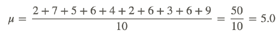
Step 2: Calculate the mean of the data values.
Step 3: Calculate the differences between the data values and the mean. Enter the results in the second column.
| x | (x−μ) |
|---|---|
| 2 | −3 |
| 7 | 2 |
| 5 | 0 |
| 6 | 1 |
| 4 | −1 |
| 2 | −3 |
| 6 | 1 |
| 3 | −2 |
| 6 | 1 |
| 9 | 4 |
Step 4: Calculate the values for column 3 by squaring each result in the second column.
| (x−μ)2 |
|---|
| 9 |
| 4 |
| 0 |
| 1 |
| 1 |
| 9 |
| 1 |
| 4 |
| 1 |
| 16 |
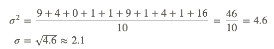
Step 5: Calculate the mean of the third column and then take the square root of the answer. This value is the standard deviation (σ) of the data set.
Step 5 can be written using the formula
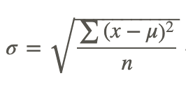
The standard deviation of the data set is approximately 2.1.
Now that you have completed all the steps, here is the table that was used to record the results. The table was separated as the steps were completed. Now that you know the process involved in calculating the standard deviation, there is no need to work with individual columns−work with an entire table.
| x | (x−μ) | (x−μ)2 |
|---|---|---|
| 2 | −3 | 9 |
| 7 | 2 | 4 |
| 5 | 0 | 0 |
| 6 | 1 | 1 |
| 4 | −1 | 1 |
| 2 | −3 | 9 |
| 6 | 1 | 1 |
| 3 | −2 | 4 |
| 6 | 1 | 1 |
| 9 | 4 | 16 |
Review
- The following data was collected. 71737769806778777082 Fill in the chart below and calculate the standard deviation. The data represents a small population.
| Data (x) | Mean (μ) | Data − Mean (x−μ) | Square of Data − Mean (x−μ)2 | |
|---|---|---|---|---|
| ∑ |
- The following data was collected: 5548657048596744 Fill in the chart below and calculate the standard deviation. The data represents a sample.
| Data (x) | Mean (x¯) | Data − Mean (x−x¯) | Square of Data − Mean (x−x¯)2 | |
|---|---|---|---|---|
| ∑ |
- Suppose data are normally distributed, with a mean of 100 and a standard deviation of 20. Between what 2 values will approximately 68% of the data fall?
a. 60 and 140
b. 80 and 120
c. 20 and 100
d. 100 and 125 - The sum of all of the deviations about the mean of a set of data is always going to be equal to:
a. positive
b. the mode
c. the standard deviation total
d. 0 - Suppose data are normally distributed, with a mean of 50 and a standard deviation of 10. Between what 2 values will approximately 95% of the data fall?
a. 40 and 60
b. 30 and 70
c. 20 and 80
d. 10 and 95 - If data are normally distributed, what percentage of the data should lie within the range of μ±3σ?
a. 34%
b. 68%
c. 95%
d. 99.7% - If a normally distributed population has a mean of 75 and a standard deviation of 15, what proportion of the values would be expected to lie between 45 and 105?
a. 34%
b. 68%
c. 95%
d. 99.7% - If a normally distributed population has a mean of 25 and a standard deviation of 5.5, what proportion of the values would be expected to lie between 19.5 and 30.5?
a. 34%
b. 68%
c. 95%
d. 99.7% - In the United States, cola can normally be bought in 8 oz cans. A survey was conducted where 250 cans of cola were taken from a manufacturing warehouse and the volumes were measured. It was found that the mean volume was 7.5 oz, and the standard deviation was 0.1 oz. Draw a normal distribution curve to represent this data and then answer the following questions.
a. 68% of the volumes can be found between __________ and _________.
b. 95% of the volumes can be found between __________ and _________.
c. 99.7% of the volumes can be found between __________ and _________. - The mean height of the fourth graders in a local elementary school was found to be 4’8”, or 56”. The standard deviation was found to be 5”. Draw a normal distribution curve to represent this data and then answer the following questions.
a. 68% of the heights can be found between __________ and _________.
b. 95% of the heights can be found between __________ and _________.
c. 99.7% of the heights can be found between __________ and _________.
Vocabulary
| Term | Definition |
|---|---|
| inflection point | An inflection point is a point in the domain where concavity changes from positive to negative or negative to positive. |
| 68-95-99.7 Rule | When 68% of the data values would be located within 1 standard deviation of the mean, 95% of the data values would be located within 2 standard deviations of the mean, and 99.7% of the data values would be located within 3 standard deviations of the mean, statisticians refer to this as the 68-95-99.7 Rule. |
| standard deviation | The square root of the variance is the standard deviation. Standard deviation is one way to measure the spread of a set of data. |
| variance | A measure of the spread of the data set equal to the mean of the squared variations of each data value from the mean of the data set. |
Additional Resources
PLIX: Play, Learn, Interact, eXplore - Variance of a Data Set
Video: Standard Deviation of a Normally Distributed Data Set
Activities: Standard Deviation of a Data Set Discussion Questions
Lesson Plans: Calculating the Standard Deviation Lesson Plan
Practice: Standard Deviation of a Data Set
Real World: Variance of a Data Set