
10.6: Non-Parametric Statistics
- Page ID
- 5802
Non-Parametric Analytical Methods
Situations Where We Use Non-Parametric Tests
If non-parametric tests have fewer assumptions and can be used with a broader range of data types, why don’t we use them all the time? The reason is because there are several advantages of using parametric tests. They are more robust and have greater power, which means that they have a greater chance of rejecting the null hypothesis relative to the sample size when the null hypothesis is false.
However, parametric tests demand that the data meet stringent requirements, such as normality and homogeneity of variance.
For example, a one-sample t-test requires that the sample be drawn from a normally distributed population. When testing two independent samples, not only is it required that both samples be drawn from normally distributed populations, but it is also required that the standard deviations of the populations be equal. If either of these conditions is not met, our results are not valid.
As mentioned, an advantage of non-parametric tests is that they do not require the data to be normally distributed. In addition, although they test the same concepts, non-parametric tests sometimes have fewer calculations than their parametric counterparts. Non-parametric tests are often used to test different types of questions and allow us to perform analysis with categorical and rank data. The table below lists the parametric tests, their non-parametric counterparts, and the purpose of each test.
Commonly Used Parametric and Non-parametric Tests
| Parametric Test (Normal Distributions) | Non-parametric Test (Non-normal Distributions) | Purpose of Test |
|---|---|---|
| t-test for independent samples | Rank sum test | Compares means of two independent samples |
| Paired t-test | Sign test | Examines a set of differences of means |
| Pearson correlation coefficient | Rank correlation test | Assesses the linear association between two variables. |
| One-way analysis of variance (F-test) | Kruskal-Wallis test | Compares three or more groups |
| Two-way analysis of variance | Runs test | Compares groups classified by two different factors |
The Sign Test
One of the simplest non-parametric tests is the sign test. The sign test examines the difference in the medians of matched data sets. It is important to note that we use the sign test only when testing if there is a difference between the matched pairs of observations. This test does not measure the magnitude of the relationship-it simply tests whether the differences between the observations in the matched pairs are equally likely to be positive or negative. Many times, this test is used in place of a paired t-test.
For example, we would use the sign test when assessing if a certain drug or treatment had an impact on a population or if a certain program made a difference in behavior. We first determine whether there is a positive or negative difference between each of the matched pairs. To determine this, we arrange the data in such a way that it is easy to identify what type of difference that we have. Let’s take a look at an example to help clarify this concept.
Performing a Sign Test
Suppose we have a school psychologist who is interested in whether or not a behavior intervention program is working. He examines 8 middle school classrooms and records the number of referrals written per month both before and after the intervention program. Below are his observations:
| Observation Number | Referrals Before Program | Referrals After Program |
|---|---|---|
| 1 | 8 | 5 |
| 2 | 10 | 8 |
| 3 | 2 | 3 |
| 4 | 4 | 1 |
| 5 | 6 | 4 |
| 6 | 4 | 1 |
| 7 | 5 | 7 |
| 8 | 9 | 6 |
Since we need to determine the number of observations where there is a positive difference and the number of observations where there is a negative difference, it is helpful to add an additional column to the table to classify each observation as such (see below). We ignore all zero or equal observations.
| Observation Number | Referrals Before Program | Referrals After Program | Change |
|---|---|---|---|
| 1 | 8 | 5 | − |
| 2 | 10 | 8 | − |
| 3 | 2 | 3 | + |
| 4 | 4 | 1 | − |
| 5 | 6 | 4 | − |
| 6 | 4 | 1 | − |
| 7 | 5 | 7 | + |
| 8 | 9 | 6 | − |
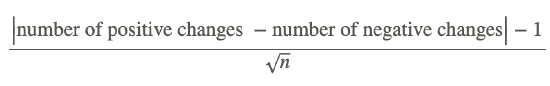
The test statistic we use is
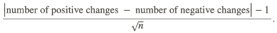
If the sample has fewer than 30 observations, we use the t-distribution to determine a critical value and make a decision. If the sample has more than 30 observations, we use the normal distribution.
Our example has only 8 observations, so we calculate our t-score as shown below:
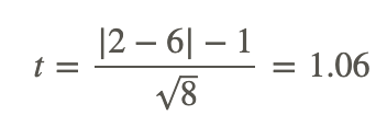
Similar to other hypothesis tests using standard scores, we establish null and alternative hypotheses about the population and use the test statistic to assess these hypotheses. As mentioned, this test is used with paired data and examines whether the medians of the two data sets are equal. When we conduct a pre-test and a post-test using matched data, our null hypothesis is that the difference between the data sets will be zero. In other words, under our null hypothesis, we would expect there to be some fluctuations between the pre-test and post-test, but nothing of significance. Therefore, our null and alternative hypotheses would be as follows:
H0:m=0
Ha:m≠0
With the sign test, we set criterion for rejecting the null hypothesis in the same way as we did when we were testing hypotheses using parametric tests. For the example above, if we set α=0.05, we would have critical values at 2.36 standard scores above and below the mean. Since our standard score of 1.06 is less than the critical value of 2.36, we would fail to reject the null hypothesis and cannot conclude that there is a significant difference between the pre-test and post-test scores.
When we use the sign test to evaluate a hypothesis about the median of a population, we are estimating the likelihood, or the probability, that the number of successes would occur by chance if there was no difference between pre-test and post-test data. When working with small samples, the sign test is actually the binomial test, with the null hypothesis being that the proportion of successes will equal 0.5.
Performing the Binomial Test
Suppose a physical education teacher is interested in the effect of a certain weight-training program on students’ strength. She measures the number of times students are able to lift a dumbbell of a certain weight before the program and then again after the program. Below are her results:
| Before Program | After Program | Change |
|---|---|---|
| 12 | 21 | + |
| 9 | 16 | + |
| 11 | 14 | + |
| 21 | 36 | + |
| 17 | 28 | + |
| 22 | 20 | − |
| 18 | 29 | + |
| 11 | 22 | + |
If the program had no effect, then the proportion of students with increased strength would equal 0.5. Looking at the data above, we see that 7 of the 8 students had increased strength after the program. But is this statistically significant? To answer this question, we use the binomial formula, which is as follows:
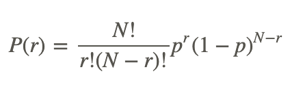
Using this formula, we need to determine the probability of having either 7 or 8 successes as shown below:
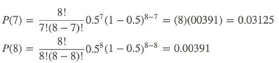
To determine the probability of having either 7 or 8 successes, we add the two probabilities together and get 0.03125+0.00391=0.0352. This means that if the program had no effect on the matched data set, we have a 0.0352 likelihood of obtaining the number of successes that we did by chance.
Using the Sign Test to Examine Categorical Data
We can also use the sign test to examine differences and evaluate hypotheses with categorical data sets. Recall that we typically use the chi-square distribution to assess categorical data. We could use the sign test when determining if one categorical variable is really more than another. For example, we could use this test if we were interested in determining if there were equal numbers of students with brown eyes and blue eyes. In addition, we could use this test to determine if equal numbers of males and females get accepted to a four-year college.
When using the sign test to examine a categorical data set and evaluate a hypothesis, we use the same formulas and methods as if we were using nominal data. The only major difference is that instead of labeling the observations as positives or negatives, we would label the observations with whatever dichotomy we want to use (male/female, brown/blue, etc.) and calculate the test statistic, or probability, accordingly. Again, we would not count zero or equal observations.
Examining Categorical Data
The UC admissions committee is interested in determining if the numbers of males and females who are accepted into four-year colleges differ significantly. They take a random sample of 200 graduating high school seniors who have been accepted to four-year colleges. Out of these 200 students, they find that there are 134 females and 66 males. Do the numbers of males and females accepted into colleges differ significantly? Since we have a large sample, calculate the z-score and use α=0.05.
To answer this question using the sign test, we would first establish our null and alternative hypotheses:
H0:mHa:m=0≠0
This null hypothesis states that the median numbers of males and females accepted into UC schools are equal.
Next, we use α=0.05 to establish our critical values. Using the normal distribution table, we find that our critical values are equal to 1.96 standard scores above and below the mean.
To calculate our test statistic, we use the following formula:
However, instead of the numbers of positive and negative observations, we substitute the number of females and the number of males. Because we are calculating the absolute value of the difference, the order of the variables does not matter. Therefore, our z-score can be calculated as shown:
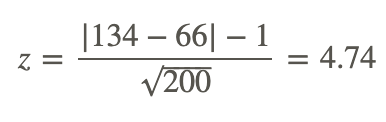
With a calculated test statistic of 4.74, we can reject the null hypothesis and conclude that there is a difference between the number of graduating males and the number of graduating females accepted into the UC schools.
The Benefit of Using the Sign Rank Test
As previously mentioned, the sign test is a quick and easy way to test if there is a difference between pre-test and post-test matched data. When we use the sign test, we simply analyze the number of observations in which there is a difference. However, the sign test does not assess the magnitude of these differences.
A more useful test that assesses the difference in size between the observations in a matched pair is the sign rank test. The sign rank test (also known as the Wilcoxon sign rank test) resembles the sign test, but it is much more sensitive. Similar to the sign test, the sign rank test is also a nonparametric alternative to the paired Student’s t-test. When we perform this test with large samples, it is almost as sensitive as Student’s t-test, and when we perform this test with small samples, it is actually more sensitive than Student’s t-test.
The main difference with the sign rank test is that under this test, the hypothesis states that the difference between observations in each data pair (pre-test and post-test) is equal to zero. Essentially, the null hypothesis states that the two variables have identical distributions. The sign rank test is much more sensitive than the sign test, since it measures the difference between matched data sets. Therefore, it is important to note that the results from the sign and the sign rank test could be different for the same data set.
To conduct the sign rank test, we first rank the differences between the observations in each matched pair, without regard to the sign of the difference. After this initial ranking, we affix the original sign to the rank numbers. All equal observations get the same rank and are ranked with the mean of the rank numbers that would have been assigned if they had varied. After this ranking, we sum the ranks in each sample and then determine the total number of observations. Finally, the one sample z-statistic is calculated from the signed ranks. For large samples, the z-statistic is compared to percentiles of the standard normal distribution.
It is important to remember that the sign rank test is more precise and sensitive than the sign test. However, since we are ranking the nominal differences between variables, we are not able to use the sign rank test to examine the differences between categorical variables. In addition, this test can be a bit more time consuming to conduct, since the figures cannot be calculated directly in Excel or with a calculator.
Example
Do female college students tend to be taller than their mothers? Following is computer output:
| N | N* | Below | Equal | Above | P | Median | |
|---|---|---|---|---|---|---|---|
| Difference | 76 | 10 | 21 | 11 | 44 | .0032 | 1.00 |
Example 1
Write the null and alternative hypotheses.
The null hypothesis would be that the heights are equal, and the alternative hypothesis would be that the female college students heights are greater:
H0:m=0
Ha:m>0
Example 2
What is the p-value?
The p-value is .0032.
Example 3
What are the parameters of the binomial distribution that would be used to determine this p-value?
n = 65 (the number above plus the number below) and the probability of success = .5, under the null hypothesis.
Example 4
What is your decision, based on this data?
The decision, based on this data, is to reject the null hypothesis. The p-value is less than both .05 and .01. Based on this data, we believe that college students tend to be taller than their mothers.
Review
- Which of the following kinds of data can be analyzed with nonparametric procedures:
- Normal
- Continuous
- Ranks
- All of the above
- In each situation, explain whether it is appropriate to use a sign test to analyze the question of interest. If it is appropriate, write the null and alternative hypotheses in words and using statistical symbols.
- Resting pulse rates are measured for n = 23 adult men. Is the median pulse rate of men equal to 76 or is it less than 76?
- Are median weights of 12 –year-old boys and 12-year-old girls the same, or are they different?
- A sample of 63 college women reports that their actual and ideal weights. The difference (actual – ideal) was positive for 28 of the women, negative for 19 others, and was the same for 16 women.
- Use a sign test to test the hypothesis that the population median difference is zero versus the alternative hypothesis that the median difference is greater than zero.
- What are the parameters of the binomial distribution that would be used to determine the p-value?
- Suppose a sample of 10 students at a university asked how much they spent on textbooks for the semester. The responses (in dollars) are 300, 425, 300, 276, 350, 299, 680, 55, 450 and 275. Consider a test of the null hypothesis that the population median amount spent is $425 versus the alternative hypothesis that the population median is less than $425.
- Write the null and alternative hypotheses using statistical notation.
- What is the value of the sample median spent?
- Use the sign test to make a decision.
- What are the parameters of the binomial distribution that would be used to determine the p-value of this test?
- You are interested in whether the median amount spent on textbooks at a University last year was $750. Write the null and alternative hypotheses for this situation.
- A researcher is interested in determining is the population median normal human body temperature is 98.6. Following is computer output:
Sign test of median = 98.6 versus < 98.6
| N | Equal | Above | P | Median | ||
|---|---|---|---|---|---|---|
| Bodytemp | 18 | 13 | 2 | 3 | .0106 | 98.2 |
a. Write the null and alternative hypotheses.
b. What is the p-value?
c. What is your decision? Explain.
- True or False? The Wilcoxon test is valid for data from any distribution, whether Normal or not.
- True or False? The Wilcoxon test is much less sensitive to outliers than the two-sample t-test.
- The following data are the resting pulse rates of 7 people who say they do not exercise and ten people who say they do exercise: Do not exercise: 74, 86, 68, 74, 64, 86, 78 Do Exercise: 64, 74, 62, 65, 77, 66, 62, 54, 66, 82
- It is believed that pulse rates of people who exercise tend to be lower than the pulse rates of those who do not exercise. With this in mind, write the null and hypothesis for a two-sample Wilcoxon test.
- Perform the Wilcoxon test.
- State a conclusion about the null and alternative hypotheses in the context of this situation.
- The following data of weight losses comes from a study of overweight people who were randomly divided into two groups – one of 7 people on a diet plan and the other of 7 people on an exercise plan. Diet plan: 12, 10, 14, 18, 2, 9, 37 Exercise plan: 14, 9, 4, 5, 7, 6, and 11
- Find the value of the Wilcoxon test statistic that would compare the two methods for losing weight.
- State a conclusion in the context of this situation.
- The following table fives the results of a 2-sample Wilcoxon test to compare the median cholesterol level of heart attack patients to the medial cholesterol of the patients who did not have a heart attack. Heart attack N=28 Median = 268.00 Control N=30 Median = 187.00 W = 1140.0 Test o eta1 = eta2 vs eta1 >eta2 Is significant at 0.0000
- State the null and alternative hypotheses.
- State a conclusion about the hypotheses. Explain based on the output in the table.
- Two drivers are testing the mileage of different models of cars. The gas mileage of nine different cars is as indicated. Use the Wilcoxon signed rank test to test at the 5% level whether there is a difference in gas for the two drivers based on the data.
| Driver 1 | Driver 2 |
|---|---|
|
16.4 |
18.8 |
| 17.0 | 19.8 |
| 29.8 | 28.2 |
| 50.8 | 49.6 |
| 18.8 | 20.3 |
| 25.7 | 30.5 |
| 34.8 | 35.1 |
| 39.3 | 46.0 |
| 46.0 | 46.0 |
- In a different test, thirty-three cars were examined. Differences in mileage were calculated and ranked. There were three differences that were equal to zero. The sum of the positive ranks was 200 and the sum of the negative ranks was 265. Use the Wilcoxon signed rank test to test at the 5% level whether there is a difference in the gas mileage for the two drivers.'
Vocabulary
| Term | Definition |
|---|---|
| Kruskal-Wallis test | The Kruskal-Wallis test is used when we are assessing the one-way variance of a specific variable in non-normal distributions. |
| non-parametric tests | Non-parametric tests are done for data that is not normally distributed and are often used to test different types of questions and allow us to perform analysis with categorical and rank data. |
| rank sum test | The rank sum test is a nonparametric test (t-test for independence) that compares means of two independent samples |
| Runs test | The runs test is a two-way ANOVA and used to compare groups classified by two different factors |
| sign rank test | The sign rank test (also known as the Wilcoxon sign rank test) and is a quick and easy way to test if there is a difference between pre-test and post-test matched data. |
| sign test | The sign test is the simplest non-parametric test where it examines the difference in the medians of matched data sets. |
Additional Resources
Video: Wilcoxon Signed-Ranks Test
Practice: Non-Parametric Statistics