
2.6.2: Translating Sine and Cosine Functions
- Page ID
- 14927
Graph shifted trig functions
Explore how changes to the equations of sine and cosine functions affect the graphs of the functions through transformations (stretches and shifts).
Warm-Up
Sine and cosine are functions that display periodic behavior when graphed. Use the interactive below to change amplitude of sine and cosine and alter their graphs. Later in this section you will see how to alter these graphs via transformation.
Add interactive element text here. This box will NOT print up in pdfs
Work it Out 1
You have seen linear, quadratic and even exponential and logarithmic functions undergo transformations to stretch and shift them. How might the graph of a periodic function behave under these types of transformations? Explore this question using the interactive below.
Add interactive element text here. This box will NOT print up in pdfs
The general equation for a sine curve is: \(y=A\sin (w(x−h))+k\). In this equation, A represents the amplitude. How does changing the value of the amplitude impact the graph of a sine function? Begin by sketching a graph of the sine function \(y=\sin (x)\). Then pick several different values for A including positive and negative values, numbers close 0, and 0 itself, and graph those equations as well. What happens to your graph as the amplitude changes?
Discussion
These are the graphs of \(y=\sin (x)\) (red) and \(y=2\sin (x)\) (green). What impact did changing A from 1 to 2 have on the graph? Predict what the graph would look like when \(A=−2\), and then graph the function. How would you compare the graphs of \(y=2\sin (x)\) and \(y=−2\sin (x)\)? In other words, does the amplitude change when A is a positive number vs. a negative number? What generalizations can you make about the relationship between the absolute value of A and the amplitude?
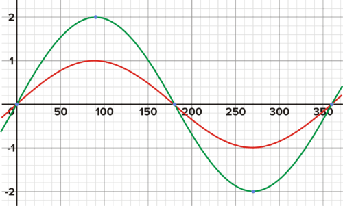
What generalizations can you make about the relationship between the absolute value of A and the amplitude?
Determine the equation for the graph below. The scale of the x-axis is in degrees.
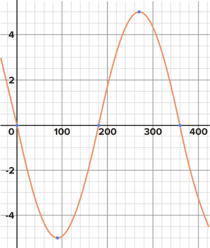
Solution
The graph is the inverse of a basic sine function, which means \(A\) is a negative number. The amplitude of the graph is at \(y=−5\) and \(y=+5\), or in other words, the minimum and maximum values on the graph are 5 away from the midline. Therefore, the equation is \(y=−5\sin (x)\).
Work it Out 2
Just as you did in the previous Active Learning, start by graphing \(y=\sin (x)\). Then experiment with different values for h including positive and negative values, and values close to 0. How do these different values for h impact the graph?
Discussion
Recall that the expression for a sine curve is \(y=A\sin (w(x−h))+k\). Therefore, when \(h\) has a positive value, it will be subtracted from x. The h represents the phase shift of the function. How is the graph impacted differently by positive and negatives phase shifts? Can you create an equation with a non-zero phase shift that would look the same when graphed as the equation \(y=\sin (x)\)?
Graph \(y=\cos \left(x−\dfrac{\pi }{4}\right)\)
Solution
This function will be shifted \(\dfrac{\pi }{4}\) units to the right. The easiest way to sketch the curve is to start with the parent graph and then move it to the right the correct number of units.
Work it Out 3
Use the same process as above to explore how a sine curve is impacted when you change the value of k, which is also called the midline or the sinusoidal axis. Pick several different values for k, including positive and negative values, to see how k affects the graph.
Discussion
The parent graph of \(y=\sin (x)\) is shifted up or down on the graph as k changes. In other words, the graph is translated \(k\) units. If \(k=1\), does the graph shift up or down? What about if \(k=−1\)?
Work it Out 4
How is the parent graph of the sine curve impacted by changing the value of \(w\), the frequency? What happens if \(w\) is a positive number \(v\). a negative number? Predict what happens if \(w\) (the frequency) is changed to both positive and negative values, as well as values between 0 and 1, and values greater than 1.
Discussion
The frequency describes the number of cycles of the graph between \(0^{\circ}\) and \(360^{\circ}\), or between \(\pi\) and \(2\pi \). When the frequency is 2, there are two cycles within this range.
Work it Out 5: Transforming the Graph of Sine Functions
Experiment with these PLIX to see the relationship between the sine function and its graph.
CK-12 INTERACTIVES
Graphing Translated Sine Functions
Without using a graphing calculator, sketch the graph of a sine function where \(A=3\), \(\dfrac{\pi }{2}\), \(w=2\), and the midline is 4.
Solution
Start by writing an equation with the values given above:
\(y=3\sin \left(2\left(x−\dfrac{\pi }{2}\right)\right)+4\)
It will be helpful to start with the parent graph and translate it one step at a time. This is the graph of the function \(y=\sin (x) \)
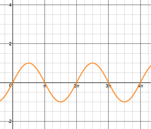
The graph of y = sin x
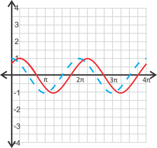
Now adjust the phase shift of the function, which shifts the graph to the left by \(\dfrac{\pi }{2}\) or \(90^{\circ}\). The blue graph below is of the function \(y=\sin \left(x−\dfrac{\pi }{2}\right)\).
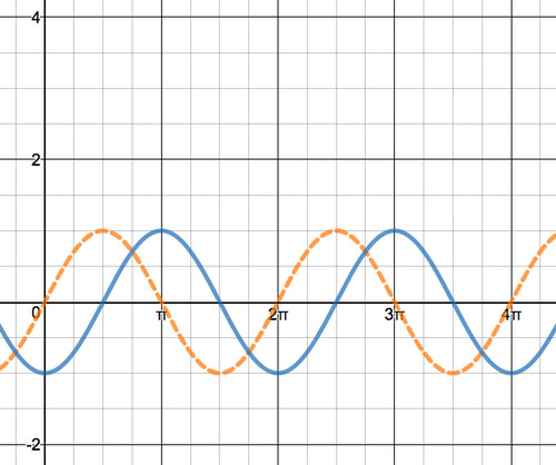
The graphs y = sin x (orange), and \(y = \sin \left(x- \dfrac{\pi}{2}\right)\) (blue)
Now adjust the midline of the function. The location of the midline is impacted by the value of k. In this example, \(k = 4\), which shifts the graph up by 4 units on the y-axis. The purple graph below is of the function \(y=\sin (x−\dfrac{\pi }{2})+4\).
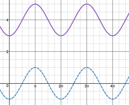
The graphs \(y = \sin \left(x - \dfrac{\pi}{2}\right)\) (blue), and \(y = \sin \left(x - \dfrac{\pi}{2}\right)+4\) (purple)
Next adjust the amplitude of the function. The amplitude of the purple graph is 1, but the new equation has an amplitude of 3, so the distance between the midline (which is now at \(y = 4\)) and the maximum and minimum y-values should be 3. Therefore, the maximum and minimum values should be at \(y = 1\) and \(y = 7\). The green graph below is for the equation: \(y=3\sin \left(x−\dfrac{\pi }{2}\right)+4\).
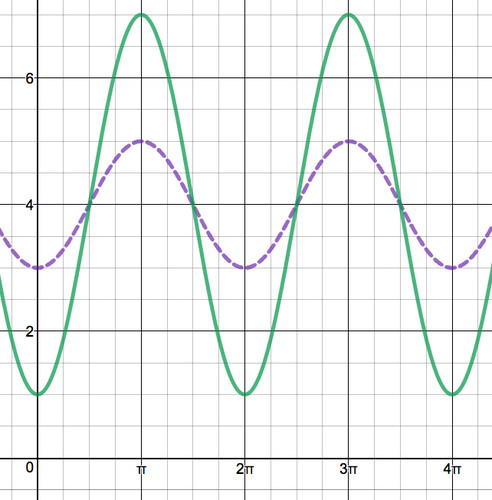
The graphs \(y = \sin \left(x - \dfrac{\pi}{2}\right)+4\) (purple) and \(y = 3\sin \left(x- \dfrac{\pi}{2}\right)+4\) (green)
Finally, you need to adjust the frequency of the graph. Because the value of \(w = 2\), the graph needs to go through 2 complete cycles between \(0^{\circ}\) and \(360^{\circ}\) or between 0 and \(2\pi \). The red graph below is of the function \(y=3\sin \left(2\left(x−\dfrac{\pi }{2}\right)\right)+4\).
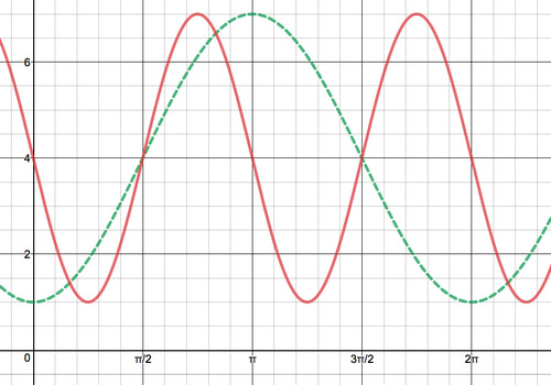
The red graph is of the function \(y=3\sin \left(2\left(x−\dfrac{\pi }{2}\right)\right)+4\).
Determining a Trigonometric Equation from a Transformed Parent Graph
Find the equation of the cosine curve below.
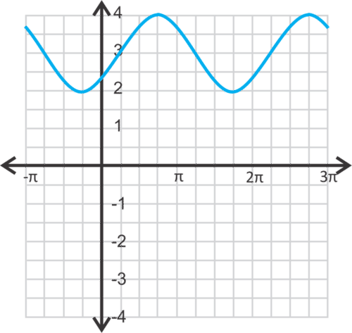
Solution
The parent graph is in green (below). It moves up 3 units (red) and then to the right 3\pi 4 units (blue). Therefore, the equation is \(y=\cos \left(x−\dfrac{3\pi }{4}\right)+3\).
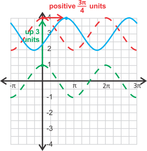
If you moved the cosine curve backward, then the equation would be \(y=\cos \left(x+\dfrac{5\pi }{4}\right)+3\).
Review
For questions 1-4, match the equation with its graph.
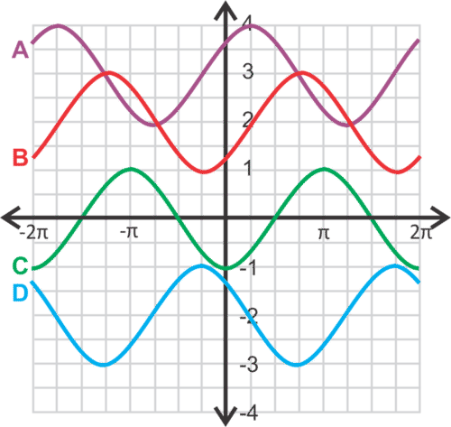
Match the Equation with the Graph.
- \(y=\sin \left(x−\dfrac{\pi }{2}\right)\)
- \(y=\cos \left(x−\dfrac{\pi }{4}\right)+3\)
- \(y=\cos \left(x+\dfrac{\pi }{4}\right)−2\)
- \(y=\sin \left(x−\dfrac{\pi }{4}\right)+2\)
Which graph above also represents these equations in #5 and #6?
- \(y=\cos \left(x−\pi \right)\)
- \(y=\sin \left(x+\dfrac{3\pi }{4}\right)−2\)
- Write another sine equation for graph A.
- Writing: How many sine (or cosine) equations can be generated for one curve? Why?
For questions 9 - 14, graph the following equations from \([−2\pi , 2\pi ]\).
- \(y=2\sin \left(x+\pi 4\right)\)
- \(y=1+\cos x\)
- \(y=\cos \left(x+\pi \right)−2\)
- \(y=\sin \left(x−\dfrac{\pi}{6} \right)\)
- \(y=\cos \left(3(x−1)\right)−3\)
- Critical Thinking: Is there a difference between \(y=\sin x+1\) and \(y=\sin (x+1)\)? Explain your answer.