K12 LibreTexts

5.1.1: Plots of Polar Coordinates

  • Page ID
    4195
  • \( \newcommand{\vecs}[1]{\overset { \scriptstyle \rightharpoonup} {\mathbf{#1}} } \)

    \( \newcommand{\vecd}[1]{\overset{-\!-\!\rightharpoonup}{\vphantom{a}\smash {#1}}} \)

    \( \newcommand{\id}{\mathrm{id}}\) \( \newcommand{\Span}{\mathrm{span}}\)

    ( \newcommand{\kernel}{\mathrm{null}\,}\) \( \newcommand{\range}{\mathrm{range}\,}\)

    \( \newcommand{\RealPart}{\mathrm{Re}}\) \( \newcommand{\ImaginaryPart}{\mathrm{Im}}\)

    \( \newcommand{\Argument}{\mathrm{Arg}}\) \( \newcommand{\norm}[1]{\| #1 \|}\)

    \( \newcommand{\inner}[2]{\langle #1, #2 \rangle}\)

    \( \newcommand{\Span}{\mathrm{span}}\)

    \( \newcommand{\id}{\mathrm{id}}\)

    \( \newcommand{\Span}{\mathrm{span}}\)

    \( \newcommand{\kernel}{\mathrm{null}\,}\)

    \( \newcommand{\range}{\mathrm{range}\,}\)

    \( \newcommand{\RealPart}{\mathrm{Re}}\)

    \( \newcommand{\ImaginaryPart}{\mathrm{Im}}\)

    \( \newcommand{\Argument}{\mathrm{Arg}}\)

    \( \newcommand{\norm}[1]{\| #1 \|}\)

    \( \newcommand{\inner}[2]{\langle #1, #2 \rangle}\)

    \( \newcommand{\Span}{\mathrm{span}}\) \( \newcommand{\AA}{\unicode[.8,0]{x212B}}\)

    \( \newcommand{\vectorA}[1]{\vec{#1}}      % arrow\)

    \( \newcommand{\vectorAt}[1]{\vec{\text{#1}}}      % arrow\)

    \( \newcommand{\vectorB}[1]{\overset { \scriptstyle \rightharpoonup} {\mathbf{#1}} } \)

    \( \newcommand{\vectorC}[1]{\textbf{#1}} \)

    \( \newcommand{\vectorD}[1]{\overrightarrow{#1}} \)

    \( \newcommand{\vectorDt}[1]{\overrightarrow{\text{#1}}} \)

    \( \newcommand{\vectE}[1]{\overset{-\!-\!\rightharpoonup}{\vphantom{a}\smash{\mathbf {#1}}}} \)

    \( \newcommand{\vecs}[1]{\overset { \scriptstyle \rightharpoonup} {\mathbf{#1}} } \)

    \( \newcommand{\vecd}[1]{\overset{-\!-\!\rightharpoonup}{\vphantom{a}\smash {#1}}} \)

    \(\newcommand{\avec}{\mathbf a}\) \(\newcommand{\bvec}{\mathbf b}\) \(\newcommand{\cvec}{\mathbf c}\) \(\newcommand{\dvec}{\mathbf d}\) \(\newcommand{\dtil}{\widetilde{\mathbf d}}\) \(\newcommand{\evec}{\mathbf e}\) \(\newcommand{\fvec}{\mathbf f}\) \(\newcommand{\nvec}{\mathbf n}\) \(\newcommand{\pvec}{\mathbf p}\) \(\newcommand{\qvec}{\mathbf q}\) \(\newcommand{\svec}{\mathbf s}\) \(\newcommand{\tvec}{\mathbf t}\) \(\newcommand{\uvec}{\mathbf u}\) \(\newcommand{\vvec}{\mathbf v}\) \(\newcommand{\wvec}{\mathbf w}\) \(\newcommand{\xvec}{\mathbf x}\) \(\newcommand{\yvec}{\mathbf y}\) \(\newcommand{\zvec}{\mathbf z}\) \(\newcommand{\rvec}{\mathbf r}\) \(\newcommand{\mvec}{\mathbf m}\) \(\newcommand{\zerovec}{\mathbf 0}\) \(\newcommand{\onevec}{\mathbf 1}\) \(\newcommand{\real}{\mathbb R}\) \(\newcommand{\twovec}[2]{\left[\begin{array}{r}#1 \\ #2 \end{array}\right]}\) \(\newcommand{\ctwovec}[2]{\left[\begin{array}{c}#1 \\ #2 \end{array}\right]}\) \(\newcommand{\threevec}[3]{\left[\begin{array}{r}#1 \\ #2 \\ #3 \end{array}\right]}\) \(\newcommand{\cthreevec}[3]{\left[\begin{array}{c}#1 \\ #2 \\ #3 \end{array}\right]}\) \(\newcommand{\fourvec}[4]{\left[\begin{array}{r}#1 \\ #2 \\ #3 \\ #4 \end{array}\right]}\) \(\newcommand{\cfourvec}[4]{\left[\begin{array}{c}#1 \\ #2 \\ #3 \\ #4 \end{array}\right]}\) \(\newcommand{\fivevec}[5]{\left[\begin{array}{r}#1 \\ #2 \\ #3 \\ #4 \\ #5 \\ \end{array}\right]}\) \(\newcommand{\cfivevec}[5]{\left[\begin{array}{c}#1 \\ #2 \\ #3 \\ #4 \\ #5 \\ \end{array}\right]}\) \(\newcommand{\mattwo}[4]{\left[\begin{array}{rr}#1 \amp #2 \\ #3 \amp #4 \\ \end{array}\right]}\) \(\newcommand{\laspan}[1]{\text{Span}\{#1\}}\) \(\newcommand{\bcal}{\cal B}\) \(\newcommand{\ccal}{\cal C}\) \(\newcommand{\scal}{\cal S}\) \(\newcommand{\wcal}{\cal W}\) \(\newcommand{\ecal}{\cal E}\) \(\newcommand{\coords}[2]{\left\{#1\right\}_{#2}}\) \(\newcommand{\gray}[1]{\color{gray}{#1}}\) \(\newcommand{\lgray}[1]{\color{lightgray}{#1}}\) \(\newcommand{\rank}{\operatorname{rank}}\) \(\newcommand{\row}{\text{Row}}\) \(\newcommand{\col}{\text{Col}}\) \(\renewcommand{\row}{\text{Row}}\) \(\newcommand{\nul}{\text{Nul}}\) \(\newcommand{\var}{\text{Var}}\) \(\newcommand{\corr}{\text{corr}}\) \(\newcommand{\len}[1]{\left|#1\right|}\) \(\newcommand{\bbar}{\overline{\bvec}}\) \(\newcommand{\bhat}{\widehat{\bvec}}\) \(\newcommand{\bperp}{\bvec^\perp}\) \(\newcommand{\xhat}{\widehat{\xvec}}\) \(\newcommand{\vhat}{\widehat{\vvec}}\) \(\newcommand{\uhat}{\widehat{\uvec}}\) \(\newcommand{\what}{\widehat{\wvec}}\) \(\newcommand{\Sighat}{\widehat{\Sigma}}\) \(\newcommand{\lt}{<}\) \(\newcommand{\gt}{>}\) \(\newcommand{\amp}{&}\) \(\definecolor{fillinmathshade}{gray}{0.9}\)

    Points as distance from the origin and angle from an axis.

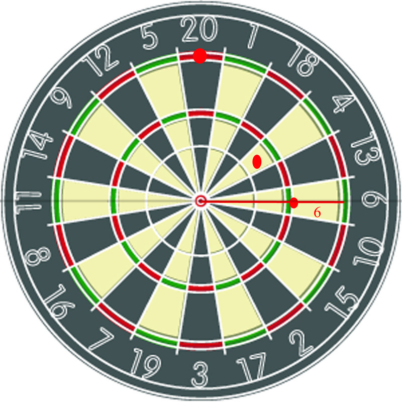
    While playing a game of darts with your friend, you decide to see if you can plot the coordinates of where your darts land. The dartboard looks like this
    f-d_9e0a62da9f90b25f7369b9975ca4dc95df01840bc4eccd46a425a2de+IMAGE_TINY+IMAGE_TINY.jpg
    Figure \(\PageIndex{1}\)

    While trying to set up a rectangular coordinate system, your friend tells you that it would be easier to plot the positions of your darts using a ‘‘polar coordinate system’’. Can you do this?

    Plots of Polar Coordinates

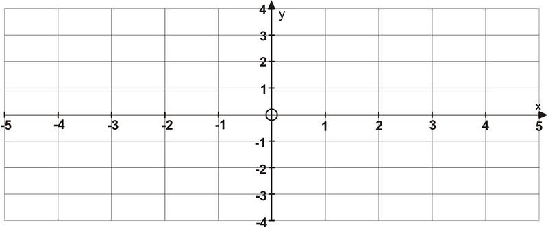
    The graph paper that you have used for plotting points and sketching graphs has been rectangular grid paper. All points were plotted in a rectangular form \((x,y)\) by referring to a set of perpendicular \(x\)− and \(y\)− axes. In this section you will discover an alternative to graphing on rectangular grid paper – graphing on circular grid paper.

    Look at the two options below:
    f-d_16a6ce1e77fc838f684185efc9a6abf4666096badbb16091a6838f3d+IMAGE_TINY+IMAGE_TINY.jpg
    Figure \(\PageIndex{2}\)
    f-d_494f460c9e0397dd3cd1c21a4a64f0021eeabb895c928253a3854c52+IMAGE_TINY+IMAGE_TINY.jpg
    Figure \(\PageIndex{3}\)

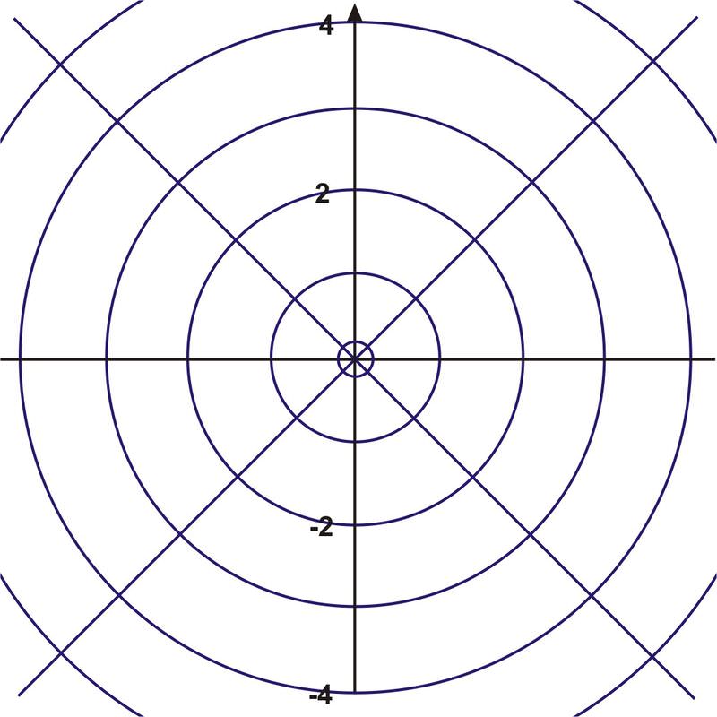
    You are all familiar with the rectangular grid paper shown above. However, the circular paper lends itself to new discoveries. The paper consists of a series of concentric circles-circles that share a common center. The common center \(O\), is known as the pole or origin and the polar axis is the horizontal line \(r\) that is drawn from the pole in a positive direction. The point \(P\) that is plotted is described as a directed distance \(r\) from the pole and by the angle that \(\overline{OP} \) makes with the polar axis. The coordinates of \(P\) are \((r,\theta )\).

    These coordinates are the result of assuming that the angle is rotated counterclockwise. If the angle were rotated clockwise then the coordinates of \(P\) would be \((r,−\theta )\). These values for \(P\) are called polar coordinates and are of the form \(P(r,\theta )\) where \(r\) is the absolute value of the distance from the pole to \(P\) and \(\theta \) is the angle formed by the polar axis and the terminal arm \(\overline{OP} \).

    Plotting Points

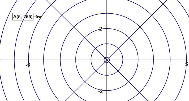
    Plot the point \(A(5,−255^{\circ})\) and the point \(B(3,60^{\circ})\).

    To plot A, move from the pole to the circle that has \(r=5\) and then rotate \(255^{\circ}\) clockwise from the polar axis and plot the point on the circle. Label it \(A\).
    f-d_88ed5575d8f31fbbba07b559fc4d7755540fe8ec19694220336ee710+IMAGE_TINY+IMAGE_TINY.jpg
    Figure \(\PageIndex{4}\)

    To plot B, move from the pole to the circle that has \(r=3\) and then rotate \(60^{\circ}\) counter clockwise from the polar axis and plot the point on the circle. Label it \(B\).
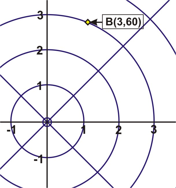
    f-d_dd5f561df21fa82461fe76b59d96476670801d0100d12fa025aa2cc7+IMAGE_TINY+IMAGE_TINY.jpg
    Figure \(\PageIndex{5}\)

    Determining Pairs of Polar Coordinates

    Determine four pairs of polar coordinates that represent the following point \(P(r,\theta )\) such that \(−360^{\circ}\leq \theta \leq 360^{\circ}\).
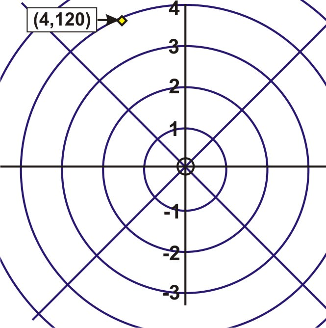
    f-d_5202ddf283bab2d1fefeb440c11ec077117f5c6fb4cc84272fea2f46+IMAGE_TINY+IMAGE_TINY.jpg
    Figure \(\PageIndex{6}\)

    Pair 1 \(\rightarrow (4,120^{\circ})\). Pair 2 \(\rightarrow (4,−240^{\circ})\) comes from using \(k=−1\) and \((r,\theta +360^{\circ}k)\),(4,120^{\circ}+360(−1)). Pair 3 \(\rightarrow (−4,300^{\circ})\) comes from using \(k=0\) and \((−r,\theta +[2k+1]180^{\circ}),(−4,120^{\circ}+[2(0)+1]180^{\circ})\). Pair 4 \(\rightarrow (−4,−60^{\circ})\) comes from using \(k=−1\) and \((−r,\theta +[2k+1]180^{\circ})\),\((−4,120^{\circ}+[2(−1)+1]180^{\circ})\).

    Plotting Polar Coordinates

    Plot the following coordinates in polar form and give their description in polar terms: \((1,0)\), \((0,1)\), \((-1,0)\), \((-1,1)\).
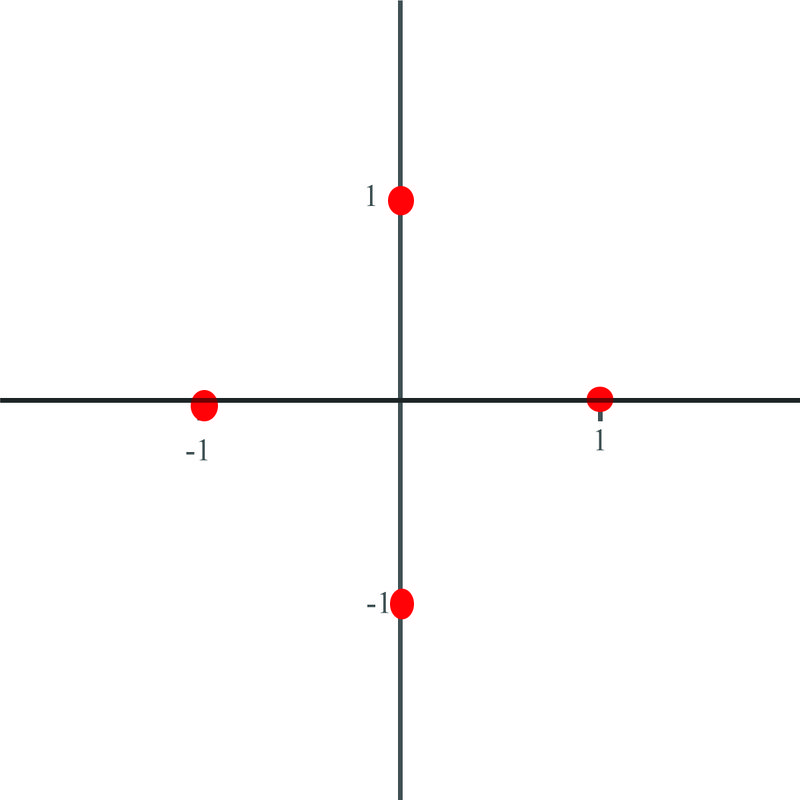
    f-d_68a601b0213d43f830ff588a21f2ab1e71d614065c54cbf9f235d2cb+IMAGE_TINY+IMAGE_TINY.jpg
    Figure \(\PageIndex{7}\)

    The points plotted are shown above. Since each point is 1 unit away from the origin, we know that the radius of each point in polar form will be equal to 1.

    The first point lies on the positive 'x' axis, so the angle in polar coordinates is \(0^{\circ}\). The second point lies on the positive 'y' axis, so the angle in polar coordinates is \(90^{\circ}\). The third point lies on the negative 'x' axis, so the angle in polar coordinates is \(180^{\circ}\). The fourth point lies on the negative 'y' axis, so the angle in polar coordinates is \(270^{\circ}\).

    Example \(\PageIndex{1}\)

    Earlier, you were asked to plot the positions of your darts using a polar coordinate system.

    Since you have the positions of the darts on the board with both the distance from the origin and the angle they make with the horizontal, you can describe them using polar coordinates.
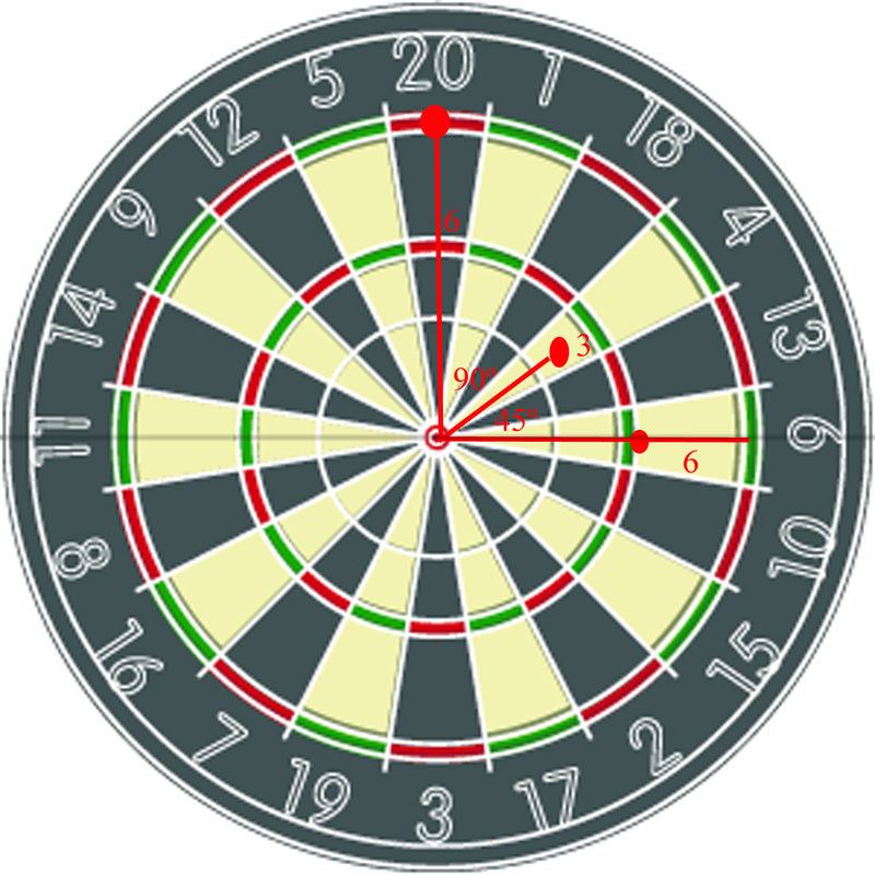
    f-d_962fbb3e41e25d03805bfbe9151733b52f295485d25e04e4e265eaac+IMAGE_TINY+IMAGE_TINY.jpg
    Figure \(\PageIndex{8}\)

    Solution

    As you can see, the positions of the darts are:

    \((3,45^{\circ} )\), \((6,90^{\circ} )\)

    and

    \((4,0^{\circ} )\)

    Example \(\PageIndex{2}\)

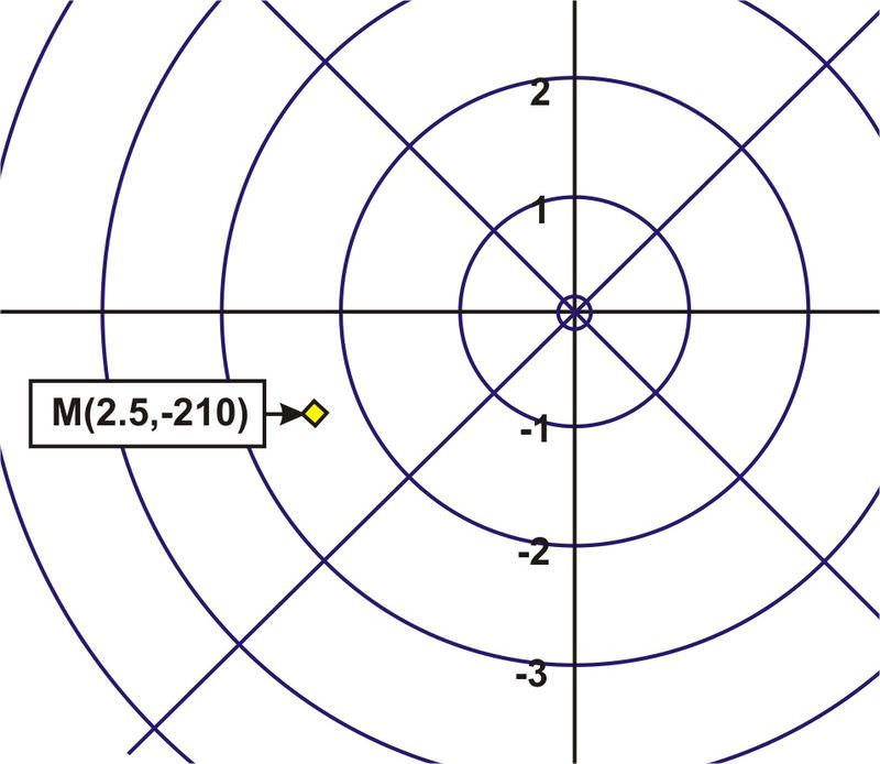
    Plot the point \(M\left(2.5, 210^{\circ} \right)\).

    Solution
    f-d_a5e63e3f6002f1c6987660f0678e2a1b8840f57b3bfcadb51a73eaa1+IMAGE_TINY+IMAGE_TINY.jpg
    Figure \(\PageIndex{9}\)
    Example \(\PageIndex{3}\)

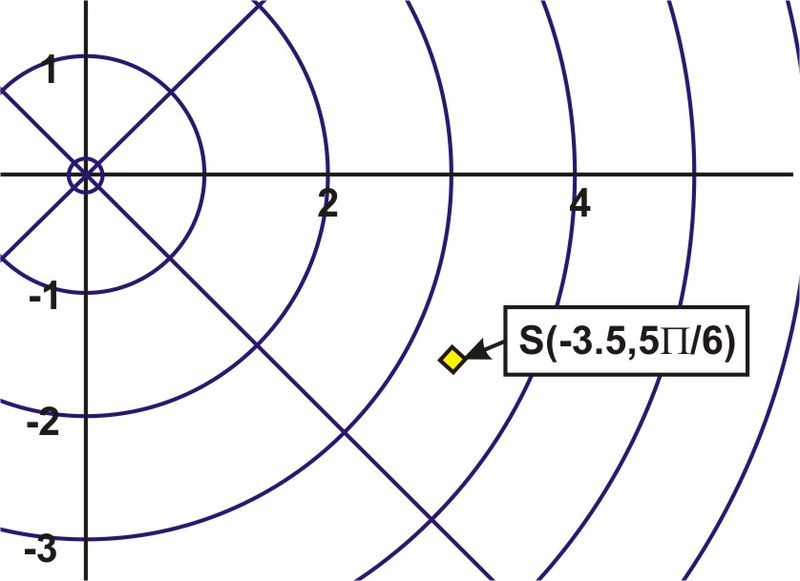
    Plot the point \(S\left(−3.5,\dfrac{5\pi }{6}\right)\).

    Solution
    f-d_8a81dbe93124bff1f6faa836a4b2287ea4742e3c553a9ca318edf29f+IMAGE_TINY+IMAGE_TINY.jpg
    Figure \(\PageIndex{10}\)
    Example \(\PageIndex{4}\)

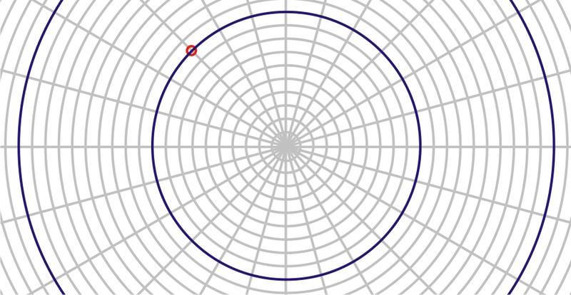
    Plot the point \(A\left(1, \dfrac{3\pi }{4}\right)\).

    Solution
    f-d_e8fae6c569ca0fdbb50d0acb1a207e463a97188fde914ceb88c73ddb+IMAGE_TINY+IMAGE_TINY.jpg
    Figure \(\PageIndex{11}\)

    Review

    Plot the following points on a polar coordinate grid.

    1. \((3,150^{\circ})\)
    2. \((2,90^{\circ})\)
    3. \((5,60^{\circ})\)
    4. \((4,120^{\circ})\)
    5. \((3,210^{\circ})\)
    6. \((−2,120^{\circ})\)
    7. \((4,−90^{\circ})\)
    8. \((−5,−30^{\circ})\)
    9. \((2,−150^{\circ})\)
    10. \((−3,300^{\circ})\)

    Give three alternate sets of coordinates for the given point within the range \(−360^{\circ}\leq \theta \leq 360^{\circ}\).

    1. \((3,60^{\circ})\)
    2. \((2,210^{\circ})\)
    3. \((4,330^{\circ})\)
    4. Find the length of the arc between the points \((2,30^{\circ})\) and \((2,90^{\circ})\).
    5. Find the area of the sector created by the origin and the points \((4,30^{\circ})\) and \((4,90^{\circ})\).

    Review (Answers)

    To see the Review answers, open this PDF file and look for section 6.1.

    Additional Resources

    Interactive Element

    Video: Polar Coordinates 1


    This page titled 5.1.1: Plots of Polar Coordinates is shared under a CK-12 license and was authored, remixed, and/or curated by CK-12 Foundation via source content that was edited to the style and standards of the LibreTexts platform.

    CK-12 Foundation
    LICENSED UNDER
    CK-12 Foundation is licensed under CK-12 Curriculum Materials License
    • Was this article helpful?