5.1.3: Graph Polar Equations

Points and graphs based on equations involving radius and angle measurements.

In the rectangular coordinate system, points are identified by their distances from the x and y axes. In the polar coordinate system, points are identified by their angle on the unit circle and their distance from the origin. You can use basic right triangle trigonometry to translate back and forth between the two representations of the same point. How are lines and other functions affected by this new coordinate system?

Polar and Rectangular Coordinates

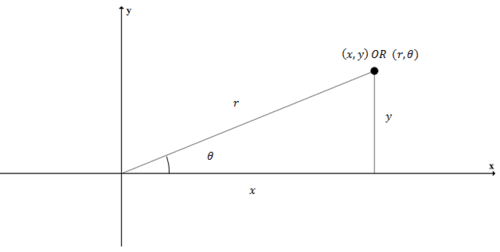
Rectangular coordinates are the ordinary \((x,y)\) coordinates that you are used to.

Figure \(\PageIndex{1}\)

Polar coordinates represent the same point, but describe the point by its distance from the origin (\(r\)) and its angle on the unit circle (\(\theta \)). To translate back and forth between polar and rectangular coordinates you should use the basic trig relationships:

\(\begin{array}{l}
\sin \theta=\dfrac{y}{r} \rightarrow r \cdot \sin \theta=y \\
\cos \theta=\dfrac{x}{r} \rightarrow r \cdot \cos \theta=x \\
\tan \theta=\dfrac{y}{x} \rightarrow \theta=\tan ^{-1} \dfrac{y}{x}
\end{array}\)

You can also express the relationship between \(x\), \(y\) and \(r\) using the Pythagorean Theorem.

\(x^2+y^2=r^2\)

Note that coordinates in polar form are not unique. This is because there are an infinite number of coterminal angles that point towards any given \((x,\; y)\) coordinate.

For example, the point (3, 4) can be written in polar coordinates in at least three different ways. To find \(\theta \), use the third equation from above and to find r use the pythagorean theorem.

\(\begin{aligned}
\tan \theta&=\dfrac{4}{3} \\
\theta&=\tan ^{-1}\left(\dfrac{4}{3}\right) \approx 53.1^{\circ} \\
r^{2}&=3^{2}+4^{2} \\
r&=5
\end{aligned}\)

Three equivalent polar coordinates for the point (3, 4) are:

\((5,53.1^{\circ} ),\;(5,413.1^{\circ} ),\;(−5,233.1^{\circ} )\)

Notice how the third coordinate points in the opposite direction and has a seemingly negative radius. This means go in the opposite direction of the angle.

Once you can translate back and forth between points, use the same substitutions to change equations too. A polar equation is written with the radius as a function of the angle. This means an equation in polar form should be written in the form \(r=\underline{\qquad}\).

To write an equation in polar form, use the conversion equations to substitute. For example, to convert \(y=−x+1\) to polar form make substitutions for \(y\) and \(x\). Then, solve for \(r\).

\(\begin{aligned}
r \cdot \sin \theta &=-r \cdot \cos \theta+1 \\
r \cdot \sin \theta+r \cdot \cos \theta &=1 \\
r(\sin \theta+\cos \theta) &=1 \\
r &=\dfrac{1}{\sin \theta+\cos \theta}
\end{aligned}\)

Example \(\PageIndex{1}\)

Earlier, you were asked how lines can be represented in the polar coordinate system.

Solution

The general way to express a line \(y=mx+b\) in polar form is \(r=\dfrac{b}{\sin \theta −m\cdot cos\theta }\).

Example \(\PageIndex{2}\)

Express the following equation using rectangular coordinates: \(r=\dfrac{8}{1+2 \cos\theta }\).

Solution

Use the fact that \(r=\pm \sqrt{x^{2}+y^{2}}\) and \(r \cos\theta =x\)

\(\begin{aligned}
r+2 r \cdot \cos \theta &=8 \\
\pm \sqrt{x^{2}+y^{2}}+2 x &=8 \\
\pm \sqrt{x^{2}+y^{2}} &=8-2 x \\
x^{2}+y^{2} &=64-32 x+4 x^{2} \\
-3 x^{2}+32 x+y^{2}-64 &=0
\end{aligned}\)

This is the equation of a hyperbola.

Example \(\PageIndex{3}\)

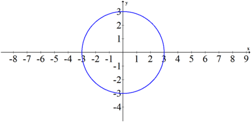
Sketch the following polar equation: \(r=3\).

Solution

Since theta is not in the equation, it can vary freely. This simple equation produces a perfect circle of radius 3 centered at the origin.

You can show this equation is equivalent to \(x^2+y^2=9\)

Figure \(\PageIndex{2}\)

Example \(\PageIndex{4}\)

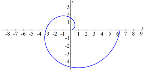
Sketch the following polar equation: \(r=\theta \) with \(\theta :0\leq\theta \leq2\pi \).

Solution

The equation r=\theta is an example of a polar equation that cannot be easily expressed in rectangular form. In order to sketch the graph, identify a few key points: \((0,0)\), \(\left(\dfrac{\pi}{2},\dfrac{\pi}{2}\right)\), \(\left(\pi ,\pi \right)\),\(\left(\dfrac{3 \pi}{2},\dfrac{3 \pi}{2}\right)\), \(\left(2\pi ,2\pi \right)\). You should see that the shape is very recognizable as a spiral.

Figure \(\PageIndex{3}\)

Example \(\PageIndex{5}\)

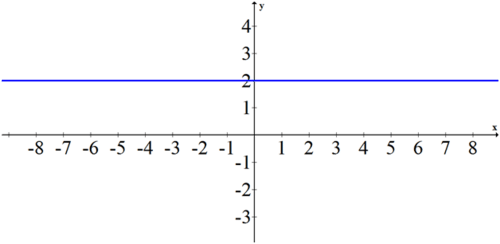
Translate the following polar expression into rectangular coordinates and then graph.

\(r=2\cdot \sec \left(\theta −\dfrac{\pi }{2}\right)\)

Solution

Simplify the polar equation first before converting to rectangular coordinates.

\(\begin{aligned}r &=2\cdot \sec\left(\theta −\dfrac{\pi }{2}\right)\\ r\cdot \cos\left(\theta −\dfrac{\pi }{2}\right)&=2 \\ r\cdot cos(\dfrac{\pi}{2}−\theta ) &=2\\ r\cdot \sin \theta &=2\\ y&=2\end{aligned}\)

Figure \(\PageIndex{4}\)

Review

Plot the following polar coordinates.

1. \(\left(3, \dfrac{5\pi }{6}\right)\)

2. \(\left(2, \dfrac{\pi }{2}\right)\)

3. \(\left(4, \dfrac{−7\pi }{6}\right)\)

4. \(\left(−2, \dfrac{5\pi }{3}\right)\)

Give two alternate sets of coordinates for each point.

5. \((2,60^{\circ} )\)

6. \((5,330^{\circ} )\)

7. \((2,210^{\circ} )\)

Graph each equation.

8. \(r=4\)

9. \(\theta =\dfrac{\pi }{4}\)

10. \(r=2\theta \) with \(\theta : 0\leq\theta \leq2\pi \).

Convert each point to rectangular form.

11. \(\left(4, \dfrac{2\pi }{3}\right)\)

12. \(\left(3, \dfrac{\pi }{4}\right)\)

13. \((5, \dfrac{\pi }{3})\)

Convert each point to polar form using radians where \(0\leq\theta <2\pi \).

14. (1, 3)

15. (1, -4)

16. (2, 6)

Convert each equation to polar form.

17. \(x=3\)

18. \(2x+4y=2\)

Review (Answers)

To see the Review answers, open this PDF file and look for section 10.1.

Vocabulary

Term	Definition
Coterminal Angles	A set of coterminal angles are angles with the same terminal side but expressed differently, such as a different number of complete rotations around the unit circle or angles being expressed as positive versus negative angle measurements.
polar coordinate system	The polar coordinate system is a special coordinate system in which the location of each point is determined by its distance from the pole and its angle with respect to the polar axis.
polar coordinates	Polar coordinates describe locations on a grid using the polar coordinate system. The location of each point is determined by its distance from the pole and its angle with respect to the polar axis.
rectangular coordinates	A point is written using rectangular coordinates if it is written in terms of x and y and can be graphed on the Cartesian plane.
unit circle	The unit circle is a circle of radius one, centered at the origin.

Additional Resources

Video: Graphing Polar Equations - Overview

Practice: Graph Polar Equations

Real World: Listen Up