5.1.5: Special Polar Equations and Graphs
- Page ID
- 4199
Archimedean spirals, cardioids, and roses.
Max is in charge of the sound system for his big sister’s wedding reception. He can’t get into the hall until the morning of the wedding, so he’s going to have to set up his microphones and speakers in record time. He does, however, have a floor plan of the hall. How can he make sure that the pick-up areas of the microphones and the broadcast area of the speakers don’t overlap and cause feedback? He’ll have time for some minimal trial and error, but he needs to have a general idea where all the microphones and speakers will be during the reception. Can he use polar coordinates to help him place his equipment?
More Polar Equations and Graphs
Why do people continue to use polar coordinates when modern computers are powerful and fast enough to solve extremely complicated problems in rectangular form? One reason is that many polar graphs are beautiful and intriguing. Polar graphs can help people see patterns that they might otherwise overlook. Artists have even used polar graphs as the basis of their designs.
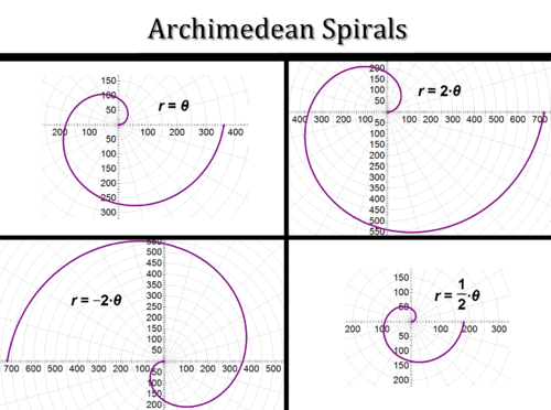
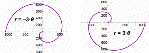
One of the simplest equations that forms a special polar curve is \(r=a\theta \), where a is any real number and \theta ranges from zero to infinity. Equations of this form create a shape known as an Archimedean spiral. As \(\theta \) increases, the graph continues to spiral out like a perfect snail’s shell. The following graphs demonstrate how changing the value of a alters the spiral. Note that each curve will continue to spiral forever.
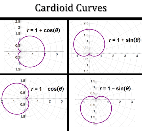
Another important polar curve is the cardioid. People who work with acoustics know that the cardioid is an accurate model for both the pick-up range of certain types of microphones and the broadcast range for certain kinds of speakers. Cardioids get their name from their heart-like shapes. Equations of the form \(r=1+a\cos \theta \) produce cardioid curves. You can change the orientation of a cardioid, or of any other polar equation with cosine in its standard form, by replacing cosine with sine, negative cosine, or negative sine.
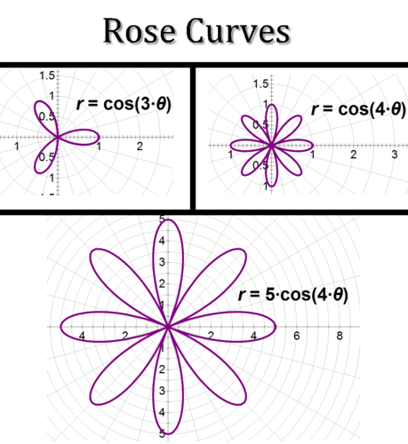
Rose curves are another interesting set of polar curves. For these equations of the form \(r=a\cos n\theta \), where \(n\) is a natural number, the plots resemble flowers. When \(n\) is odd, the flowers have \(n\) petals, and when n is even, the flowers have \(2n\) petals.
You can use your graphing calculator or other technology to help you graph all of these polar curves.
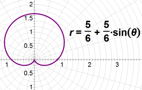
With this knew information, what is the shape of the graph of the polar equation \(6r=5+5\sin\theta \)?
First, isolate \(r\) to get \(r=\dfrac{5}{6}+\dfrac{5}{6}\sin\theta \). This graph appears most similar to the cardioid curve, which is \(r=1+a\cos \theta \). However, the changes to the form mean that the graph will be rotated by \(\dfrac{\pi }{2}\) and slightly smaller than the standard cardioid. Now, graph the equation to test the predictions.
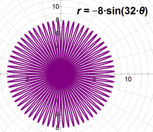
Now, let's describe the graph of \(r=−8\sin(32\theta )\), then graph it.
This graph matches the format for a rose curve: \(r=a\cos n\theta \). Since n is even the final graph should have 64 petals. The – sine means that the graph will be rotated \(−\dfrac{\pi }{2}\) radians from its starting position.
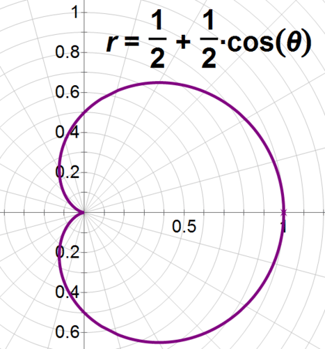
Earlier, you were asked how Max can set up the sound system for his sister's wedding so that the speakers don't overlap. Max can use cardioids to help him set up the sound system without causing feedback. He researches his microphones and speakers online and finds out that the pick-up pattern of his microphones can be graphed using the equation \(r=\dfrac{1}{2}+\dfrac{1}{2}\cos \theta \). Since he has multiple microphones to place, he can graph the curve and use it with his floor plan to ensure that the mikes don’t overlap and that he places the speakers in the dead zones behind the microphones, where they won’t pick up any sound.
Solution
Since the microphones pick up along the polar axis between 0 and 1, he’ll want to position speakers in the dead zone, where \(r<0\), and \(\theta =0\). He can also position speakers at other places in the dead zone, but cardioid microphones are least likely to pick up sound when it’s \pi radians from their optimal pick-up areas.
Describe what the graph \(r=−3\theta \) will look like. Then, change the equation to rotate it by \(\pi \) radians. Graph the original and rotated graphs.
Solution
The graph will make an Archimedean spiral three times larger than the normal one. To rotate the graph, change the -3 to 3.
For each of the following examples, identify the polar curve given by the equation and then graph it.
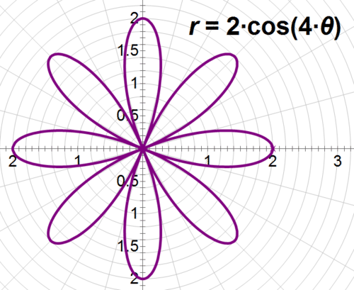
\(6\cos 4\theta −3r=0\)
Solution
First, solve for \(r\). Then, identify the equation.
\(\begin{aligned} 6\cos 4\theta −3r &=0\\ 3r&=6\cos 4\theta \\ r&=2\cos 4\theta \end{aligned}\)
The graph will be of a rose curve with 8 petals.
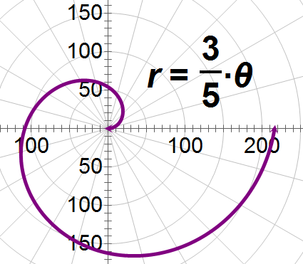
\(5r=3\theta\)
Solution
First, solve for \(r\). Then, identify the equation.
\(\begin{aligned} 5r &=3\theta \\ r&=\dfrac{3}{5} \theta \end{aligned}\)
The graph will be Archimedean spiral.
\(5r−25+45\cos 3\theta =0\)
Solution
First, solve for \(r\). Then, identify the equation.
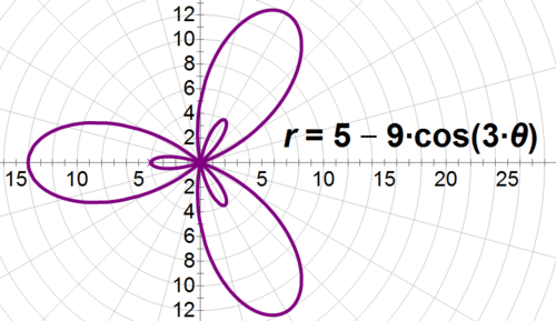
\(\begin{aligned} 5r−25+45\cos 3\theta &=0 \\ 5r&=25−45\cos 3\theta \\ r&=5−9\cos 3\theta\end{aligned}\)
At first glance, this equation looks similar to a cardioid. However, it also has \(n\theta \) like a rose curve. You’ll have to graph it to get a good sense for what the combination does - it’s a rose curve within a rose curve!
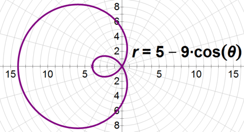
However, take out the three, graph \(r=5−9\cos \theta \), and you’ll get a curve similar to a cardioid curve. This equation illustrates how small changes can produce complicated, beautiful, polar graphs.
Review
For #1-3, describe the family of equations that produces that curve.
- Rose curve
- Archimedean spiral
- Cardioid curve
For #4-15, identify the polar curve and then graph it.
- \(\dfrac{r}{2}=\theta\)
- \(r=1−4\cos \theta\)
- \(3r=4\cos (8\theta )\)
- \(r=\dfrac{1}{2}+\dfrac{1}{2}\cos (\theta )\)
- \(r=−\theta\)
- \(\dfrac{r}{4}=4\cos (4\theta )\)
- \(r=−4\theta\)
- \(r=−2\\sin (8\theta )\)
- \(r=1−\\sin \theta\)
- \(1=\cos \theta +r\)
- \(r=5\)
- \(r=5\theta\)
Review (Answers)
To see the Review answers, open this PDF file and look for section 10.12.
Vocabulary
| Term | Definition |
|---|---|
| Archimedean spiral | An Archimedean spiral is a pattern that resembles a snail shell. It’s formed by equations in the r=a\theta family. |
| cardioid | A cardioid curve is a polar graph formed by variations on the equation \(r=1+a\cos \theta \), where a is a real number. Cardioid curves are heart-shaped. They're especially important for people who work in acoustics and sound design, \since they model the performance of many microphones and speakers. |
| rose | A rose curve is a polar curve that has captivated artists and designers. It’s formed by equations in the r=a\cos n\theta family. The coefficient n is a natural number that determines the number of petals on the graph. When n is odd, the graph has n petals. When n is even, the graph has 2n petals. |
Additional Resources
Real World: Spirals in the Sea

