
7.2: Direct Imaging
- Page ID
- 5635
\( \newcommand{\vecs}[1]{\overset { \scriptstyle \rightharpoonup} {\mathbf{#1}} } \)
\( \newcommand{\vecd}[1]{\overset{-\!-\!\rightharpoonup}{\vphantom{a}\smash {#1}}} \)
\( \newcommand{\dsum}{\displaystyle\sum\limits} \)
\( \newcommand{\dint}{\displaystyle\int\limits} \)
\( \newcommand{\dlim}{\displaystyle\lim\limits} \)
\( \newcommand{\id}{\mathrm{id}}\) \( \newcommand{\Span}{\mathrm{span}}\)
( \newcommand{\kernel}{\mathrm{null}\,}\) \( \newcommand{\range}{\mathrm{range}\,}\)
\( \newcommand{\RealPart}{\mathrm{Re}}\) \( \newcommand{\ImaginaryPart}{\mathrm{Im}}\)
\( \newcommand{\Argument}{\mathrm{Arg}}\) \( \newcommand{\norm}[1]{\| #1 \|}\)
\( \newcommand{\inner}[2]{\langle #1, #2 \rangle}\)
\( \newcommand{\Span}{\mathrm{span}}\)
\( \newcommand{\id}{\mathrm{id}}\)
\( \newcommand{\Span}{\mathrm{span}}\)
\( \newcommand{\kernel}{\mathrm{null}\,}\)
\( \newcommand{\range}{\mathrm{range}\,}\)
\( \newcommand{\RealPart}{\mathrm{Re}}\)
\( \newcommand{\ImaginaryPart}{\mathrm{Im}}\)
\( \newcommand{\Argument}{\mathrm{Arg}}\)
\( \newcommand{\norm}[1]{\| #1 \|}\)
\( \newcommand{\inner}[2]{\langle #1, #2 \rangle}\)
\( \newcommand{\Span}{\mathrm{span}}\) \( \newcommand{\AA}{\unicode[.8,0]{x212B}}\)
\( \newcommand{\vectorA}[1]{\vec{#1}} % arrow\)
\( \newcommand{\vectorAt}[1]{\vec{\text{#1}}} % arrow\)
\( \newcommand{\vectorB}[1]{\overset { \scriptstyle \rightharpoonup} {\mathbf{#1}} } \)
\( \newcommand{\vectorC}[1]{\textbf{#1}} \)
\( \newcommand{\vectorD}[1]{\overrightarrow{#1}} \)
\( \newcommand{\vectorDt}[1]{\overrightarrow{\text{#1}}} \)
\( \newcommand{\vectE}[1]{\overset{-\!-\!\rightharpoonup}{\vphantom{a}\smash{\mathbf {#1}}}} \)
\( \newcommand{\vecs}[1]{\overset { \scriptstyle \rightharpoonup} {\mathbf{#1}} } \)
\(\newcommand{\longvect}{\overrightarrow}\)
\( \newcommand{\vecd}[1]{\overset{-\!-\!\rightharpoonup}{\vphantom{a}\smash {#1}}} \)
\(\newcommand{\avec}{\mathbf a}\) \(\newcommand{\bvec}{\mathbf b}\) \(\newcommand{\cvec}{\mathbf c}\) \(\newcommand{\dvec}{\mathbf d}\) \(\newcommand{\dtil}{\widetilde{\mathbf d}}\) \(\newcommand{\evec}{\mathbf e}\) \(\newcommand{\fvec}{\mathbf f}\) \(\newcommand{\nvec}{\mathbf n}\) \(\newcommand{\pvec}{\mathbf p}\) \(\newcommand{\qvec}{\mathbf q}\) \(\newcommand{\svec}{\mathbf s}\) \(\newcommand{\tvec}{\mathbf t}\) \(\newcommand{\uvec}{\mathbf u}\) \(\newcommand{\vvec}{\mathbf v}\) \(\newcommand{\wvec}{\mathbf w}\) \(\newcommand{\xvec}{\mathbf x}\) \(\newcommand{\yvec}{\mathbf y}\) \(\newcommand{\zvec}{\mathbf z}\) \(\newcommand{\rvec}{\mathbf r}\) \(\newcommand{\mvec}{\mathbf m}\) \(\newcommand{\zerovec}{\mathbf 0}\) \(\newcommand{\onevec}{\mathbf 1}\) \(\newcommand{\real}{\mathbb R}\) \(\newcommand{\twovec}[2]{\left[\begin{array}{r}#1 \\ #2 \end{array}\right]}\) \(\newcommand{\ctwovec}[2]{\left[\begin{array}{c}#1 \\ #2 \end{array}\right]}\) \(\newcommand{\threevec}[3]{\left[\begin{array}{r}#1 \\ #2 \\ #3 \end{array}\right]}\) \(\newcommand{\cthreevec}[3]{\left[\begin{array}{c}#1 \\ #2 \\ #3 \end{array}\right]}\) \(\newcommand{\fourvec}[4]{\left[\begin{array}{r}#1 \\ #2 \\ #3 \\ #4 \end{array}\right]}\) \(\newcommand{\cfourvec}[4]{\left[\begin{array}{c}#1 \\ #2 \\ #3 \\ #4 \end{array}\right]}\) \(\newcommand{\fivevec}[5]{\left[\begin{array}{r}#1 \\ #2 \\ #3 \\ #4 \\ #5 \\ \end{array}\right]}\) \(\newcommand{\cfivevec}[5]{\left[\begin{array}{c}#1 \\ #2 \\ #3 \\ #4 \\ #5 \\ \end{array}\right]}\) \(\newcommand{\mattwo}[4]{\left[\begin{array}{rr}#1 \amp #2 \\ #3 \amp #4 \\ \end{array}\right]}\) \(\newcommand{\laspan}[1]{\text{Span}\{#1\}}\) \(\newcommand{\bcal}{\cal B}\) \(\newcommand{\ccal}{\cal C}\) \(\newcommand{\scal}{\cal S}\) \(\newcommand{\wcal}{\cal W}\) \(\newcommand{\ecal}{\cal E}\) \(\newcommand{\coords}[2]{\left\{#1\right\}_{#2}}\) \(\newcommand{\gray}[1]{\color{gray}{#1}}\) \(\newcommand{\lgray}[1]{\color{lightgray}{#1}}\) \(\newcommand{\rank}{\operatorname{rank}}\) \(\newcommand{\row}{\text{Row}}\) \(\newcommand{\col}{\text{Col}}\) \(\renewcommand{\row}{\text{Row}}\) \(\newcommand{\nul}{\text{Nul}}\) \(\newcommand{\var}{\text{Var}}\) \(\newcommand{\corr}{\text{corr}}\) \(\newcommand{\len}[1]{\left|#1\right|}\) \(\newcommand{\bbar}{\overline{\bvec}}\) \(\newcommand{\bhat}{\widehat{\bvec}}\) \(\newcommand{\bperp}{\bvec^\perp}\) \(\newcommand{\xhat}{\widehat{\xvec}}\) \(\newcommand{\vhat}{\widehat{\vvec}}\) \(\newcommand{\uhat}{\widehat{\uvec}}\) \(\newcommand{\what}{\widehat{\wvec}}\) \(\newcommand{\Sighat}{\widehat{\Sigma}}\) \(\newcommand{\lt}{<}\) \(\newcommand{\gt}{>}\) \(\newcommand{\amp}{&}\) \(\definecolor{fillinmathshade}{gray}{0.9}\)Just take a picture!
Seeing is believing, so it would be ideal if we could simply point a telescope at a star and take a picture of the orbiting planets. This method is called direct imaging, and the biggest challenge is separating the light of the planet from the light of the star. The problem is that the planet is typically a billion times fainter and lost in the glare of the star.
We might imagine that a directly imaged exoplanet would look like the small point of light next to the star Gliese 229 in the Figure below, first taken in 1994 at the Palomar Observatory (left) and then observed with the Hubble Space Telescope (right) in 1995.

The bright star in the figure above is GJ 229A. At a distance of about 20 light years, this star has the distinction of being one of the 100 closest stars to the Sun. GJ 229A is an M dwarf with about 60% the mass of our Sun and it is too faint to see with the naked eye. The much fainter companion, GJ 229B, was discovered at the Palomar Observatory in 1994 and is a "sub-stellar" object that is roughly 50 times the mass of Jupiter (or 0.05 times the mass of the Sun). GJ 229B does not have enough mass for hydrogen fusion to take place in its core; the radiated energy that we see comes from the fusion of deuterium to generate helium-3. Because hydrogen-fusion is the definition of a main sequence star, GJ 229B is not a star. This object is an example of a "brown dwarf" - it falls in between the upper mass limit for a planet (about 12 times the mass of Jupiter) and the lower mass limit for a star (about 70 times the mass of Jupiter). GJ 229B was the second brown dwarf to ever be discovered (the first was Teide 1) and the first brown dwarf to be discovered orbiting a star.
Naming Stars and Planets
The naming of stars seems to be one of the more disorganized efforts by astronomers. Before the age of the internet (1990's), global communication was much less efficient and astronomers worked at remote mountaintop observatories. A key task for astronomers in the early to mid 1900's was the measurement of sky coordinates and brightness of stars. Naturally, the brightest stars were cataloged independently by several different astronomers. For example, the bright star Tau Ceti has 45 different identifiers: in the Harvard Revised Bright Star Catalog it is called HR 509, in the Henry Draper catalog it is HD 10700, the Gliese Jahreiss catalog lists the star as GJ 71 and so on... The online SIMBAD site tracks this messy nomenclature, listing all of the star names and other information about individual stars for astronomers.
About half of the stars in our galaxy are gravitationally bound as binary stars that orbit a common center of mass. Some catalogs gave each of the stars their own number, while other catalogs designated the brighter star as "A" and the fainter star as "B." Sometimes, fainter components were discovered long after the catalogs were published, like GJ 229B. The discovers renamed GJ 229 as GJ 229A and they called the fainter object GJ 229B. And sometimes there are 3 or more stars (A, B, C and so on) that are gravitationally bound.
When a planet is discovered around a star it is designated with a lower case letter, starting with "b" (there are no planets with the letter "a"). Planets are named in the order that they are discovered, which makes for a confusing alphabet soup of identifiers. If the companion to GJ 229 had been a planet instead of a brown dwarf, it would have been GJ 229b.
As a side note, if you decide to "name a star" through the Star Register, you won't find your star name in any database used by astronomers (the Star Register will keep your star name in a vault and pocket your $34.99).
The picture of GJ 229B can help us to understand why direct imaging of a planet is so difficult. This brown dwarf companion is similar in size to Jupiter but emits 600 times more energy (thanks to the deuterium fusion in its core). The projected physical separation of GJ 229 A and B is similar to the Sun-Pluto distance in our solar system. If GJ 229B had been located at the Sun-Jupiter distance (5 AU) it would not have been visible in this image because it would have been completely lost in the glare of the host star.

In the image of GJ 229A taken at the 200-inch Palomar telescope, the images of GJ 229A and B have been blurred by the atmosphere of the Earth. As a point of light from a distant star enters our atmosphere, it is bent in slightly different directions a thousand times each second by turbulent blobs in our atmosphere that have slightly different indices of refraction (caused by differences in temperature or pressure). To our eyes, this appears as the romantic "twinkling" of starlight, but with even a short 1-second exposure at a telescope, the recorded image of a star is smeared.
The advantage of the Hubble Space Telescope (HST) is that the observatory is now above the Earth's atmosphere. However, even the HST image of GJ 229 is blurred by scattering of starlight on the telescope mirror and by the optics in the camera so that the final image is spread out into a speckled halo. Any planets would be comparable in brightness to the speckles and lost in the scattered image of the star. This tendency for the optical interfaces in an instrument to spread the light from a point source into a disk is called the "point spread function" (PSF) of the instrument. If the PSF of an instrument has been well-characterized, the original underlying image can be recovered to some extent by post-processing with sophisticated software analysis.
Measuring angular separations
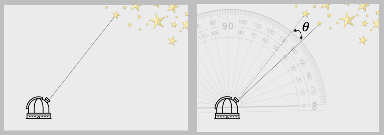
A telescope points through angles of right ascension (parallel to the lines of latitude on the Earth) and declination (parallel to lines of longitude), reading angular positions on the sky similar to the way that a protractor works as shown in the figure below. A protractor measures in units of degrees. However, one degree on the sky is an enormous distance (the angular diameter of the moon is a half a degree). One degree can be subdivided into 60 arcminutes and one arcminute can be further divided into 60 arcseconds (notationally: 1∘=60′=3600").
In astronomy, angular separations are the measurable quantity and can only be related to a linear or physical size if we know the distance to the object.
Measuring Distances - the distance to the Moon
The moon is one of the closest objects to the Earth - how do we know the distance to the moon (~240,000 miles)? There are a few ways to figure this out. First, we know that the moon completes one orbit about the Earth in 29 days, so we could apply Newton's law of gravity to relate the orbital period and the mass of the Earth to the semi-major axis of the moon's orbit about the Earth.
Aristarchus (3rd century BC) knew the diameter of the Earth and he used geometry and the angular size of the Earth's shadow relative to the apparent size of the moon during a lunar eclipse to estimate the physical size of the moon.

The most precise measurement of the distance to the moon has been made with a laser ranging experiment. Retroreflectors were placed on the surface of the moon during the NASA Apollo and Soviet Lunokhod missions. By timing the round-trip light travel time between the Earth and moon, the distance to the moon can be measured with great precision.
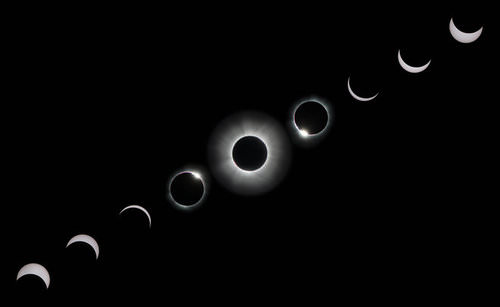
Coincidentally, the angular diameter of the sun is also a half degree (or 30 arcminutes), about the same as the angular size of the moon. The sun is physically 400 times larger than the moon, but it is also 400 times farther away than the moon. This fortuitous scaling means that when the moon passes between our line of sight to the sun, it will completely block our view of the sun for a few minutes (the figure below shows the Moon blocking out the sun during a solar eclipse).
Distances to the stars
Measuring the distances to the stars cannot be done with laser ranging. Instead, we use trigonometric parallaxes (discussed in Chapter 3.1):
Small angle approximation
We can use trigonometric functions from geometry to relate the angular size of an object to it's physical size, once we know the distance. In the figure below, the sine of the angle subtended by the moon is defined as the linear size divided by the distance to the moon. Because this is a small angle, the sine is approximately the same as the tangent of this angle.

You might worry that the sin or tan functions only apply to right angles, in which case we should be talking about \(\frac{\theta}{2}\) in the image above. However, this factor of two drops out when the radius is used instead of the diameter. Sine and tangent functions can also be represented by Taylor-Maclaurin expansions where the higher order terms drop out for small angles. When \(\theta\) is a small angle:
\[\sin\theta\sim\tan\theta\sim\theta\]
\[\text{angular separation [arcseconds]}\,=\frac{\text{separation}\,[AU]}{\text{distance [parsec]}}\]
\[\alpha\text{[arcsec]}\,=\frac{r[AU]}{d\text{[parsec]}\]
The small angle approximation works for measuring distances with parallax angles. It also works for measuring angular separations. If we know the distance to an object, angular separations can be used to derive the physical diameter of objects, like the moon in the figure above. With a known distance, angular separations are also important for monitoring the orbits of binary star systems where both stars are bright enough to be visible. Since the two stars in a binary system are both at the same distance from our solar system, if that distance is known it is easy to convert the angular separation (in arcseconds) into a physical separation (measured in AU).
Consider the case of a star at a distance of 10 parsecs with a directly imaged planet at a projected angular separation, \(\theta\,=0."5\). Solving equation 3 above, the physical separation of two stars (or a star and a visible planet) can be calculated:
distance[parsecs] ∗ angular separation[arcsec] = physical separation[AU]
10 parsec ∗ 0."5 = 5 AU
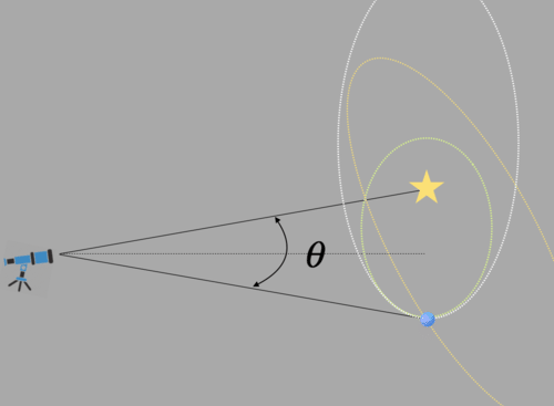
However, what does that physical separation tell us? As illustrated in the Figure below, it is just the projected separation of the stars. Keep in mind that a single measurement of 5 AU for the star-planet separation does not necessarily correspond to any parameter of the orbit. There are an infinite number of orbits that could pass through the planet position with the star at the focus of an elliptical orbit. Several measurements must be taken over time so that the time stamps on the changing positions can be used to derive the orbit of the planet.
Adaptive Optics
To obtain direct images of exoplanets around nearby stars with ground based telescopes, a technique called adaptive optics (AO) has been developed to correct for the atmospheric twinkling of starlight. This idea was first proposed in 1953 by an astronomer, Horace Babcock. However, it took the significant technological development of the Regan-era Strategic Defense Initiative (popularized as the "Star Wars" initiative) to ultimately make AO viable for astronomy.
AO combines optics, electrical engineering and computers to correct for atmospheric distortion. In cases where there is more than one star in the field of view of the telescope, light from one of the nearby bright non-science stars is picked off with a mirror and sent to the AO system. Hundreds of actuators on a deformable mirror in the AO system are pistoned at high speed (thousands of Hertz) until the image of the star is concentrated into the smallest possible point of light. This counteracts the atmospheric distortion for all stars in the field of view, including the science star of interest. The figure below shows a series of images of the star Arcturus obtained with (left to right) a "long" exposure of a a few seconds, a short exposure (a millisecond snapshot) and the AO-corrected image taken by Claire Max and her team at Lick Observatory. The AO-corrected image is similar to the image of the star that could be obtained from space.

In some cases, there are not any bright stars in the field that can be used for the AO correction. In these cases, a laser guide star is created in the upper atmosphere. Pioneered at the Lick Observatory near San Jose, California, a sodium laser is strapped to the side of the telescope and fires a narrow beam of laser light where ever the telescope points. The laser light is absorbed by a thin layer of sodium atoms about 60 miles above the ground and these atoms re-emit the light, creating an artificial star for the AO system. In the figure below, some of the sodium laser light scatters off particles in the atmosphere, giving the appearance of a light saber.

Once the image has been corrected for atmospheric blurring by an adaptive optics system, astronomers can use a coronograph to block out the light from the star and expose long enough to see the faint orbiting planets. Conceptually, this is similar to trying to see a faint object (like a tennis ball, coming over the net) that is lost in the glare of the Sun. If you use your hand to cover the Sun, you can now see the tennis ball. If you were lucky enough to be in the path of totality under clear skies during the solar eclipse of 2017, then you had the perfect demonstration of how a coronograph works. In this case, the moon acted as a coronograph, allowing people to see stars close to the Sun in the "day" sky.
At the Keck telescope in Hawai'i, astronomers used the AO system with a coronograph to detect four planets orbiting the star HR 8799. This star was selected as a good target because it is relatively close (about 40 parsecs from the Sun) and because the star is young (a mere 30 million years) so that any planets would also be young and luminous. Exoplanets are named with lower case letters beginning with "b" in the order that they are discovered. In the image below, planets b, c, and d were found in 2008 and planet e was discovered a few years later. It is challenging to find planets close to the star where the coronographic suppression of light is more difficult.
Once the light from the planet host star has been suppressed in this way, it is possible to obtain spectra of the pale dots of light from orbiting planets. Spectroscopy of the four planets around HR 8799 has been carried out using the Project 1640 instrument on the Palomar telescope and shows variable amounts of absorption from water, carbon monoxide, carbon dioxide and methane.

HR 8799 was also observed with the Hubble Space Telescope. The image of HR 8799 with HST (the figure below) shows that this is not an easy discovery, even from space. Significant processing was required to recover the underlying image of the planets (middle, below).

The search for exoplanets using coronographs is an exciting technique and impressive technological advances in this field are permitting the detection of smaller planets located at smaller inner working angles (i.e., closer to the star). The goal for the next 20 years is to develop space-based coronographs on large telescopes to image Earth-like planets around nearby stars and to obtain spectra to search for signatures of life.