7.7: Exoplanet Statistics
- Page ID
- 5640
\( \newcommand{\vecs}[1]{\overset { \scriptstyle \rightharpoonup} {\mathbf{#1}} } \)
\( \newcommand{\vecd}[1]{\overset{-\!-\!\rightharpoonup}{\vphantom{a}\smash {#1}}} \)
\( \newcommand{\dsum}{\displaystyle\sum\limits} \)
\( \newcommand{\dint}{\displaystyle\int\limits} \)
\( \newcommand{\dlim}{\displaystyle\lim\limits} \)
\( \newcommand{\id}{\mathrm{id}}\) \( \newcommand{\Span}{\mathrm{span}}\)
( \newcommand{\kernel}{\mathrm{null}\,}\) \( \newcommand{\range}{\mathrm{range}\,}\)
\( \newcommand{\RealPart}{\mathrm{Re}}\) \( \newcommand{\ImaginaryPart}{\mathrm{Im}}\)
\( \newcommand{\Argument}{\mathrm{Arg}}\) \( \newcommand{\norm}[1]{\| #1 \|}\)
\( \newcommand{\inner}[2]{\langle #1, #2 \rangle}\)
\( \newcommand{\Span}{\mathrm{span}}\)
\( \newcommand{\id}{\mathrm{id}}\)
\( \newcommand{\Span}{\mathrm{span}}\)
\( \newcommand{\kernel}{\mathrm{null}\,}\)
\( \newcommand{\range}{\mathrm{range}\,}\)
\( \newcommand{\RealPart}{\mathrm{Re}}\)
\( \newcommand{\ImaginaryPart}{\mathrm{Im}}\)
\( \newcommand{\Argument}{\mathrm{Arg}}\)
\( \newcommand{\norm}[1]{\| #1 \|}\)
\( \newcommand{\inner}[2]{\langle #1, #2 \rangle}\)
\( \newcommand{\Span}{\mathrm{span}}\) \( \newcommand{\AA}{\unicode[.8,0]{x212B}}\)
\( \newcommand{\vectorA}[1]{\vec{#1}} % arrow\)
\( \newcommand{\vectorAt}[1]{\vec{\text{#1}}} % arrow\)
\( \newcommand{\vectorB}[1]{\overset { \scriptstyle \rightharpoonup} {\mathbf{#1}} } \)
\( \newcommand{\vectorC}[1]{\textbf{#1}} \)
\( \newcommand{\vectorD}[1]{\overrightarrow{#1}} \)
\( \newcommand{\vectorDt}[1]{\overrightarrow{\text{#1}}} \)
\( \newcommand{\vectE}[1]{\overset{-\!-\!\rightharpoonup}{\vphantom{a}\smash{\mathbf {#1}}}} \)
\( \newcommand{\vecs}[1]{\overset { \scriptstyle \rightharpoonup} {\mathbf{#1}} } \)
\(\newcommand{\longvect}{\overrightarrow}\)
\( \newcommand{\vecd}[1]{\overset{-\!-\!\rightharpoonup}{\vphantom{a}\smash {#1}}} \)
\(\newcommand{\avec}{\mathbf a}\) \(\newcommand{\bvec}{\mathbf b}\) \(\newcommand{\cvec}{\mathbf c}\) \(\newcommand{\dvec}{\mathbf d}\) \(\newcommand{\dtil}{\widetilde{\mathbf d}}\) \(\newcommand{\evec}{\mathbf e}\) \(\newcommand{\fvec}{\mathbf f}\) \(\newcommand{\nvec}{\mathbf n}\) \(\newcommand{\pvec}{\mathbf p}\) \(\newcommand{\qvec}{\mathbf q}\) \(\newcommand{\svec}{\mathbf s}\) \(\newcommand{\tvec}{\mathbf t}\) \(\newcommand{\uvec}{\mathbf u}\) \(\newcommand{\vvec}{\mathbf v}\) \(\newcommand{\wvec}{\mathbf w}\) \(\newcommand{\xvec}{\mathbf x}\) \(\newcommand{\yvec}{\mathbf y}\) \(\newcommand{\zvec}{\mathbf z}\) \(\newcommand{\rvec}{\mathbf r}\) \(\newcommand{\mvec}{\mathbf m}\) \(\newcommand{\zerovec}{\mathbf 0}\) \(\newcommand{\onevec}{\mathbf 1}\) \(\newcommand{\real}{\mathbb R}\) \(\newcommand{\twovec}[2]{\left[\begin{array}{r}#1 \\ #2 \end{array}\right]}\) \(\newcommand{\ctwovec}[2]{\left[\begin{array}{c}#1 \\ #2 \end{array}\right]}\) \(\newcommand{\threevec}[3]{\left[\begin{array}{r}#1 \\ #2 \\ #3 \end{array}\right]}\) \(\newcommand{\cthreevec}[3]{\left[\begin{array}{c}#1 \\ #2 \\ #3 \end{array}\right]}\) \(\newcommand{\fourvec}[4]{\left[\begin{array}{r}#1 \\ #2 \\ #3 \\ #4 \end{array}\right]}\) \(\newcommand{\cfourvec}[4]{\left[\begin{array}{c}#1 \\ #2 \\ #3 \\ #4 \end{array}\right]}\) \(\newcommand{\fivevec}[5]{\left[\begin{array}{r}#1 \\ #2 \\ #3 \\ #4 \\ #5 \\ \end{array}\right]}\) \(\newcommand{\cfivevec}[5]{\left[\begin{array}{c}#1 \\ #2 \\ #3 \\ #4 \\ #5 \\ \end{array}\right]}\) \(\newcommand{\mattwo}[4]{\left[\begin{array}{rr}#1 \amp #2 \\ #3 \amp #4 \\ \end{array}\right]}\) \(\newcommand{\laspan}[1]{\text{Span}\{#1\}}\) \(\newcommand{\bcal}{\cal B}\) \(\newcommand{\ccal}{\cal C}\) \(\newcommand{\scal}{\cal S}\) \(\newcommand{\wcal}{\cal W}\) \(\newcommand{\ecal}{\cal E}\) \(\newcommand{\coords}[2]{\left\{#1\right\}_{#2}}\) \(\newcommand{\gray}[1]{\color{gray}{#1}}\) \(\newcommand{\lgray}[1]{\color{lightgray}{#1}}\) \(\newcommand{\rank}{\operatorname{rank}}\) \(\newcommand{\row}{\text{Row}}\) \(\newcommand{\col}{\text{Col}}\) \(\renewcommand{\row}{\text{Row}}\) \(\newcommand{\nul}{\text{Nul}}\) \(\newcommand{\var}{\text{Var}}\) \(\newcommand{\corr}{\text{corr}}\) \(\newcommand{\len}[1]{\left|#1\right|}\) \(\newcommand{\bbar}{\overline{\bvec}}\) \(\newcommand{\bhat}{\widehat{\bvec}}\) \(\newcommand{\bperp}{\bvec^\perp}\) \(\newcommand{\xhat}{\widehat{\xvec}}\) \(\newcommand{\vhat}{\widehat{\vvec}}\) \(\newcommand{\uhat}{\widehat{\uvec}}\) \(\newcommand{\what}{\widehat{\wvec}}\) \(\newcommand{\Sighat}{\widehat{\Sigma}}\) \(\newcommand{\lt}{<}\) \(\newcommand{\gt}{>}\) \(\newcommand{\amp}{&}\) \(\definecolor{fillinmathshade}{gray}{0.9}\)Exoplanet Statistics
Now that exoplanets have been detected, we can take stock of the types of planets that have been found. The Figure below summarizes the radial velocity detections (left) and transit detections (right). The radial velocity detections provide mass (M sini) and orbital period while the transit detections yield planet radius (relative to the radius of the star) and orbital period. Neither method has been successful at detecting planets similar to Earth and this is believed to be the result of poor sensitivity for the methods at the mass (or size) of Earth and the orbital period (or semi-major axis). An Earth analog would only induce a reflex velocity of 9 cm/s in a solar mass star and the transit probability falls off with increasing semi-major axis.
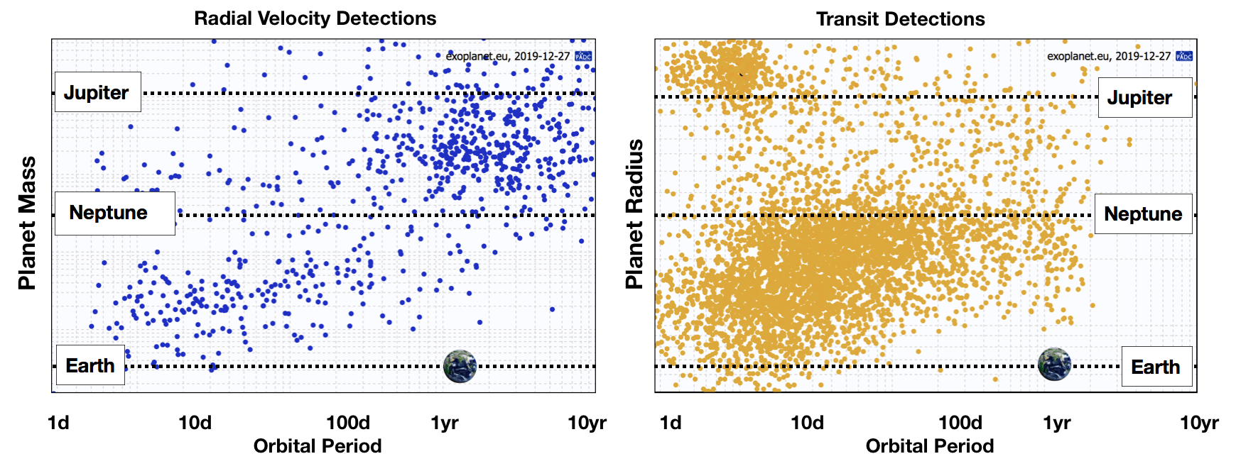
For radial velocity observations, at least one orbital period must be observed. Radial velocity surveys have been ongoing for almost 20 years, but observers tend to be impatient (it is hard to get tenure if it takes 10 years to make a discovery) and as measurement precision has improved, the focus on detecting Earth analogs has become more intense. The amplitude of the radial velocity (RV) signal depends on (1) the mass of the planet, (2) the mass of the star, and (3) the orbital period. Higher mass planets or lower mass stars produce larger radial velocity signals. The RV amplitude decreases with increasing orbital period (or increasing semi-major axis). The diagonal distribution of RV-detected planets reflects some of the observational incompleteness of this method. If RV surveys are to detect Earth analogs, the precision of this method will need to substantially improve.
For transit observations at least 3 orbital periods must be observed. The NASA Kepler mission was repurposed after 4 years. However, very few planets with orbital periods longer than about 100 days will transit because the probability of crossing the disk of the star falls off with orbital period (or semi-major axis). Because of this geometric bias, it is unlikely that transit missions will detect many Earth analogs.
The Figure below summarizes the history of planetary discovery.
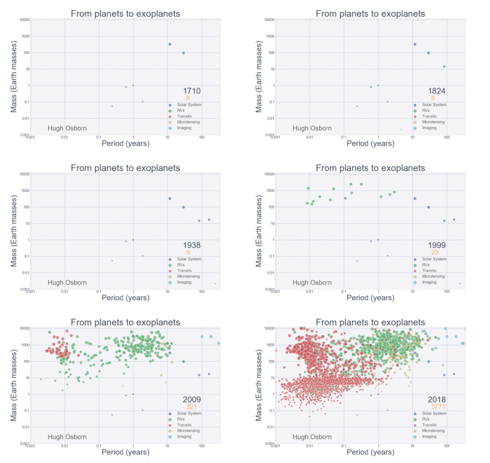
Each detection method is sensitive to a limited region of parameter space, so we cannot expect that planets would be discovered outside of the detectable region. However, there are some areas in the exoplanet parameter space where planets should have easily been detected. One region is the swath of parameter space for transiting planets with radii between Neptune (\(4R_{\oplus}\)) and Jupiter (\(10R_{\oplus}\)). The lack of planets in this region must represent a real paucity of planets.
There is also a large clump of planets similar in size or slightly larger than Jupiter, but with orbital periods shorter than 10 days among the transit detections. Some Jupiter-mass planets in short-period orbits have been found, but the RV detections seem relatively deficient in these objects. This over-abundance in short-period gas giant planets is the result of transit surveys of hundreds of thousands of stars with insufficient sensitivity to detect planets much smaller than Jupiter.
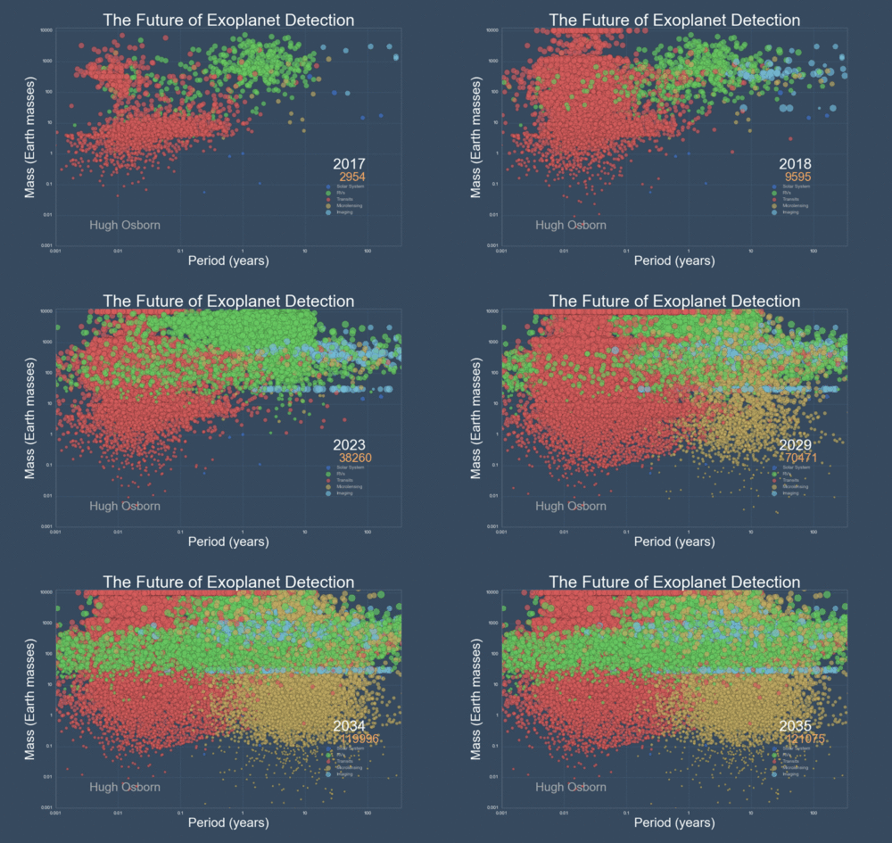
The next Figure projects a hopeful view of what discoveries should come next.
The TRAPPIST-1 system
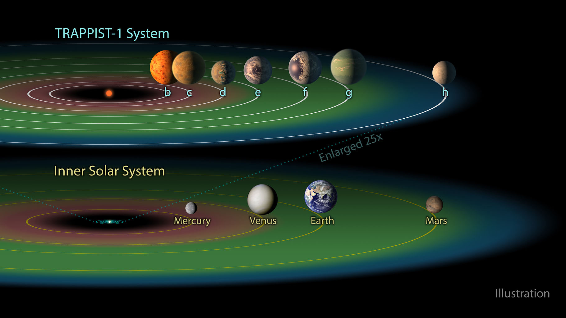
European astronomers started a program to search for exoplanets using ground-based transit photometry. Their project, with the slightly contrived name: “Transiting Planets and Planetesimals Small Telescope” or TRAPPIST, targeted M dwarf stars that are about one tenth the size of the Sun. The transit signal is proportional to the cross sectional area of the planet divided by the cross sectional area of the star, so the advantage of looking at small stars is that the transit signals from smaller planets are stronger. In 2015, three planets were detected with this survey around a star that the team renamed TRAPPIST-1 (catchier than the original catalog name for this star, 2MASS J23062928-0502285). In 2017, four more planets were discovered around this same star, bringing the total to seven planets orbiting TRAPPIST-1. All of these planets orbit at a distance that is smaller than the distance from the Sun to Mercury in our solar system and are similar in size to the rocky terrestrial worlds.
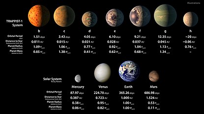
One reason that this is an intriguing system is that TRAPPIST-1 is barely a star. It has about 8% the mass of the Sun. If it were a bit smaller and TRAPPIST-1 would not even be able to fuse hydrogen and emit light. Because of its very low mass, the star burns its small reserves of hydrogen very slowly. While the Sun ends its life in another 5 billion years, TRAPPIST-1 will fuse hydrogen into helium for another 100 billion years.
Another reason that astronomers were excited about TRAPPIST-1 is that at least three of the seven planets orbit at a distance from the low luminosity star where the temperature is just right for liquid water. If there are three habitable worlds around the TRAPPIST-1 star and if technological civilizations evolve on any of these planets, there will be a powerful incentive to build spaceships that travel to these neighboring worlds.
The orbits of the seven TRAPPIST-1 planets are close to resonance, meaning that the ratio of the orbital periods are close to integer values. Planet e is in a 6-day orbit and planet g is in a 12-day orbit; planet f is in a 9.2-d orbit and planet h is in an 18.7-day orbit. This regularity in the orbits is similar to harmonics in music, and inspired a musical rendition that was mapped to the orbits of the seven TRAPPIST-1 planets.
