
1.6: The Production Possibilities Curve
- Page ID
- 1626
\( \newcommand{\vecs}[1]{\overset { \scriptstyle \rightharpoonup} {\mathbf{#1}} } \)
\( \newcommand{\vecd}[1]{\overset{-\!-\!\rightharpoonup}{\vphantom{a}\smash {#1}}} \)
\( \newcommand{\dsum}{\displaystyle\sum\limits} \)
\( \newcommand{\dint}{\displaystyle\int\limits} \)
\( \newcommand{\dlim}{\displaystyle\lim\limits} \)
\( \newcommand{\id}{\mathrm{id}}\) \( \newcommand{\Span}{\mathrm{span}}\)
( \newcommand{\kernel}{\mathrm{null}\,}\) \( \newcommand{\range}{\mathrm{range}\,}\)
\( \newcommand{\RealPart}{\mathrm{Re}}\) \( \newcommand{\ImaginaryPart}{\mathrm{Im}}\)
\( \newcommand{\Argument}{\mathrm{Arg}}\) \( \newcommand{\norm}[1]{\| #1 \|}\)
\( \newcommand{\inner}[2]{\langle #1, #2 \rangle}\)
\( \newcommand{\Span}{\mathrm{span}}\)
\( \newcommand{\id}{\mathrm{id}}\)
\( \newcommand{\Span}{\mathrm{span}}\)
\( \newcommand{\kernel}{\mathrm{null}\,}\)
\( \newcommand{\range}{\mathrm{range}\,}\)
\( \newcommand{\RealPart}{\mathrm{Re}}\)
\( \newcommand{\ImaginaryPart}{\mathrm{Im}}\)
\( \newcommand{\Argument}{\mathrm{Arg}}\)
\( \newcommand{\norm}[1]{\| #1 \|}\)
\( \newcommand{\inner}[2]{\langle #1, #2 \rangle}\)
\( \newcommand{\Span}{\mathrm{span}}\) \( \newcommand{\AA}{\unicode[.8,0]{x212B}}\)
\( \newcommand{\vectorA}[1]{\vec{#1}} % arrow\)
\( \newcommand{\vectorAt}[1]{\vec{\text{#1}}} % arrow\)
\( \newcommand{\vectorB}[1]{\overset { \scriptstyle \rightharpoonup} {\mathbf{#1}} } \)
\( \newcommand{\vectorC}[1]{\textbf{#1}} \)
\( \newcommand{\vectorD}[1]{\overrightarrow{#1}} \)
\( \newcommand{\vectorDt}[1]{\overrightarrow{\text{#1}}} \)
\( \newcommand{\vectE}[1]{\overset{-\!-\!\rightharpoonup}{\vphantom{a}\smash{\mathbf {#1}}}} \)
\( \newcommand{\vecs}[1]{\overset { \scriptstyle \rightharpoonup} {\mathbf{#1}} } \)
\(\newcommand{\longvect}{\overrightarrow}\)
\( \newcommand{\vecd}[1]{\overset{-\!-\!\rightharpoonup}{\vphantom{a}\smash {#1}}} \)
\(\newcommand{\avec}{\mathbf a}\) \(\newcommand{\bvec}{\mathbf b}\) \(\newcommand{\cvec}{\mathbf c}\) \(\newcommand{\dvec}{\mathbf d}\) \(\newcommand{\dtil}{\widetilde{\mathbf d}}\) \(\newcommand{\evec}{\mathbf e}\) \(\newcommand{\fvec}{\mathbf f}\) \(\newcommand{\nvec}{\mathbf n}\) \(\newcommand{\pvec}{\mathbf p}\) \(\newcommand{\qvec}{\mathbf q}\) \(\newcommand{\svec}{\mathbf s}\) \(\newcommand{\tvec}{\mathbf t}\) \(\newcommand{\uvec}{\mathbf u}\) \(\newcommand{\vvec}{\mathbf v}\) \(\newcommand{\wvec}{\mathbf w}\) \(\newcommand{\xvec}{\mathbf x}\) \(\newcommand{\yvec}{\mathbf y}\) \(\newcommand{\zvec}{\mathbf z}\) \(\newcommand{\rvec}{\mathbf r}\) \(\newcommand{\mvec}{\mathbf m}\) \(\newcommand{\zerovec}{\mathbf 0}\) \(\newcommand{\onevec}{\mathbf 1}\) \(\newcommand{\real}{\mathbb R}\) \(\newcommand{\twovec}[2]{\left[\begin{array}{r}#1 \\ #2 \end{array}\right]}\) \(\newcommand{\ctwovec}[2]{\left[\begin{array}{c}#1 \\ #2 \end{array}\right]}\) \(\newcommand{\threevec}[3]{\left[\begin{array}{r}#1 \\ #2 \\ #3 \end{array}\right]}\) \(\newcommand{\cthreevec}[3]{\left[\begin{array}{c}#1 \\ #2 \\ #3 \end{array}\right]}\) \(\newcommand{\fourvec}[4]{\left[\begin{array}{r}#1 \\ #2 \\ #3 \\ #4 \end{array}\right]}\) \(\newcommand{\cfourvec}[4]{\left[\begin{array}{c}#1 \\ #2 \\ #3 \\ #4 \end{array}\right]}\) \(\newcommand{\fivevec}[5]{\left[\begin{array}{r}#1 \\ #2 \\ #3 \\ #4 \\ #5 \\ \end{array}\right]}\) \(\newcommand{\cfivevec}[5]{\left[\begin{array}{c}#1 \\ #2 \\ #3 \\ #4 \\ #5 \\ \end{array}\right]}\) \(\newcommand{\mattwo}[4]{\left[\begin{array}{rr}#1 \amp #2 \\ #3 \amp #4 \\ \end{array}\right]}\) \(\newcommand{\laspan}[1]{\text{Span}\{#1\}}\) \(\newcommand{\bcal}{\cal B}\) \(\newcommand{\ccal}{\cal C}\) \(\newcommand{\scal}{\cal S}\) \(\newcommand{\wcal}{\cal W}\) \(\newcommand{\ecal}{\cal E}\) \(\newcommand{\coords}[2]{\left\{#1\right\}_{#2}}\) \(\newcommand{\gray}[1]{\color{gray}{#1}}\) \(\newcommand{\lgray}[1]{\color{lightgray}{#1}}\) \(\newcommand{\rank}{\operatorname{rank}}\) \(\newcommand{\row}{\text{Row}}\) \(\newcommand{\col}{\text{Col}}\) \(\renewcommand{\row}{\text{Row}}\) \(\newcommand{\nul}{\text{Nul}}\) \(\newcommand{\var}{\text{Var}}\) \(\newcommand{\corr}{\text{corr}}\) \(\newcommand{\len}[1]{\left|#1\right|}\) \(\newcommand{\bbar}{\overline{\bvec}}\) \(\newcommand{\bhat}{\widehat{\bvec}}\) \(\newcommand{\bperp}{\bvec^\perp}\) \(\newcommand{\xhat}{\widehat{\xvec}}\) \(\newcommand{\vhat}{\widehat{\vvec}}\) \(\newcommand{\uhat}{\widehat{\uvec}}\) \(\newcommand{\what}{\widehat{\wvec}}\) \(\newcommand{\Sighat}{\widehat{\Sigma}}\) \(\newcommand{\lt}{<}\) \(\newcommand{\gt}{>}\) \(\newcommand{\amp}{&}\) \(\definecolor{fillinmathshade}{gray}{0.9}\)Economic Models
Economists use economic models to to graphically demonstrate the concepts and theories they develop to explain human behavior and decision making.
An economy’s factors of production are scarce; they cannot produce an unlimited quantity of goods and services. A production possibilities curve is a graphical representation of the alternative combinations of goods and services an economy can produce. It illustrates the production possibilities model. In drawing the production possibilities curve, we shall assume that the economy can produce only two goods and that the quantities of factors of production and the technology available to the economy are fixed.
- Economists conduct research by evaluating sources; gathering, analyzing, and synthesizing information; and communicating conclusions supported by evidence.
- A production possibilities curve is a tool used by economists to demonstrate tradeoffs associated with allocating resources.
- What can be learned from examining a production possibilities curve?
- How can a production possibilities curve help consumers and producers make better economic choices?
Constructing a Production Possibilities Curve
To construct a production possibilities curve, we will begin with the case of a hypothetical firm, Alpine Sports, Inc., a specialized sports equipment manufacturer. Christie Ryder began the business with a single ski production facility near Killington ski resort in central Vermont. Ski sales grew, and she also saw demand for snowboards rising—particularly after snowboard competition events were included in the 2002 Winter Olympics in Salt Lake City. She added a second plant in a nearby town. The second plant, while smaller than the first, was designed to produce snowboards as well as skis. She also modified the first plant so that it could produce both snowboards and skis. Two years later she added a third plant in another town. While even smaller than the second plant, the third was primarily designed for snowboard production but could also produce skis.
We can think of each of Ms. Ryder’s three plants as a miniature economy and analyze them using the production possibilities model. We assume that the factors of production and technology available to each of the plants operated by Alpine Sports are unchanged.
Suppose the first plant, Plant 1, can produce 200 pairs of skis per month when it produces only skis. When devoted solely to snowboards, it produces 100 snowboards per month. It can produce skis and snowboards simultaneously as well.
The table in [Figure 1 - A Production Possibilities Curve] gives three combinations of skis and snowboards that Plant 1 can produce each month. Combination A involves devoting the plant entirely to ski production; combination C means shifting all of the plant’s resources to snowboard production; combination B involves the production of both goods. These values are plotted in a production possibilities curve for Plant 1. The curve is a downward-sloping straight line, indicating that there is a linear, negative relationship between the production of the two goods.
Neither skis nor snowboards is an independent or a dependent variable in the production possibilities model; we can assign either one to the vertical or to the horizontal axis. Here, we have placed the number of pairs of skis produced per month on the vertical axis and the number of snowboards produced per month on the horizontal axis.
The negative slope of the production possibilities curve reflects the scarcity of the plant’s capital and labor. Producing more snowboards requires shifting resources out of ski production and thus producing fewer skis. Producing more skis requires shifting resources out of snowboard production and thus producing fewer snowboards.
The slope of Plant 1’s production possibilities curve measures the rate at which Alpine Sports must give up ski production to produce additional snowboards. Because the production possibilities curve for Plant 1 is linear, we can compute the slope between any two points on the curve and get the same result. Between points A and B, for example, the slope equals −2 pairs of skis/snowboard (equals −100 pairs of skis/50 snowboards). (Many students are helped when told to read this result as “−2 pairs of skis per snowboard.”) We get the same value between points B and C, and between points A and C.
[Figure 1 - A Production Possibilities Curve]
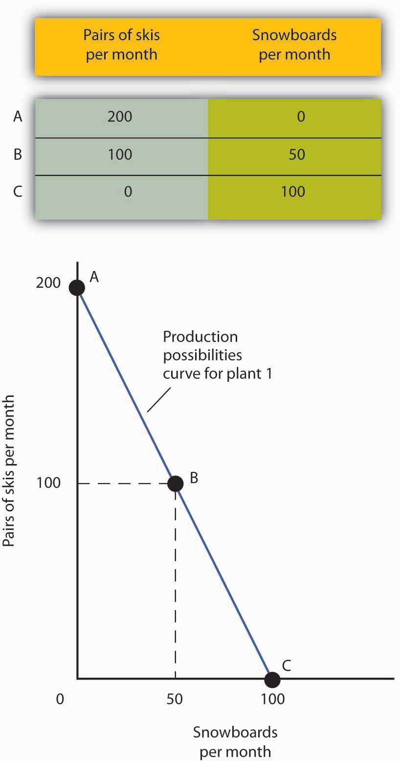
The table shows the combinations of pairs of skis and snowboards that Plant 1 is capable of producing each month. These are also illustrated with a production possibilities curve. Notice that this curve is linear.
Videos: Production Possibilities Curve and Shifting the Production Possibilities Curve
Before continuing into a more in-depth examination of the production possibilities for Alpine Sports, view the video clips below to gain a clearer understanding of the basics of the production possibilities curve:
To see this relationship more clearly, examine [Figure 2 - The Slope of a Production Possibilities Curve]. Suppose Plant 1 is producing 100 pairs of skis and 50 snowboards per month at point B. Now consider what would happen if Ms. Ryder decided to produce 1 more snowboard per month. The segment of the curve around point B is magnified in [Figure 2 - The Slope of a Production Possibilities Curve]. The slope between points B and B′ is −2 pairs of skis/snowboard. Producing 1 additional snowboard at point B′ requires giving up 2 pairs of skis. We can think of this as the opportunity cost of producing an additional snowboard at Plant 1. This opportunity cost equals the absolute value of the slope of the production possibilities curve.
![[Figure 2 - The Slope of a Production Possibilities Curve]](https://k12.libretexts.org/@api/deki/files/3706/5d95caf145e9d643d90600dd78c40f60.jpg?revision=1&size=bestfit&width=750&height=450)
[Figure 2 - The Slope of a Production Possibilities Curve]
The slope of the linear production possibilities curve in [Figure 1 - A Production Possibilities Curve] is constant; it is −2 pairs of skis/snowboard. In the section of the curve shown here, the slope can be calculated between points B and B′. Expanding snowboard production to 51 snowboards per month from 50 snowboards per month requires a reduction in ski production to 98 pairs of skis per month from 100 pairs. The slope equals −2 pairs of skis/snowboard (that is, it must give up two pairs of skis to free up the resources necessary to produce one additional snowboard). To shift from B′ to B″, Alpine Sports must give up two more pairs of skis per snowboard. The absolute value of the slope of a production possibilities curve measures the opportunity cost of an additional unit of the good on the horizontal axis measured in terms of the quantity of the good on the vertical axis that must be forgone.
The absolute value of the slope of any production possibilities curve equals the opportunity cost of an additional unit of the good on the horizontal axis. It is the amount of the good on the vertical axis that must be given up in order to free up the resources required to produce one more unit of the good on the horizontal axis. We will make use of this important fact as we continue our investigation of the production possibilities curve.
[Figure 3 - Production Possibilities at Three Plants] shows production possibilities curves for each of the firm’s three plants. Each of the plants, if devoted entirely to snowboards, could produce 100 snowboards. Plants 2 and 3, if devoted exclusively to ski production, can produce 100 and 50 pairs of skis per month, respectively. The exhibit gives the slopes of the production possibilities curves for each plant. The opportunity cost of an additional snowboard at each plant equals the absolute values of these slopes (that is, the number of pairs of skis that must be given up per snowboard).
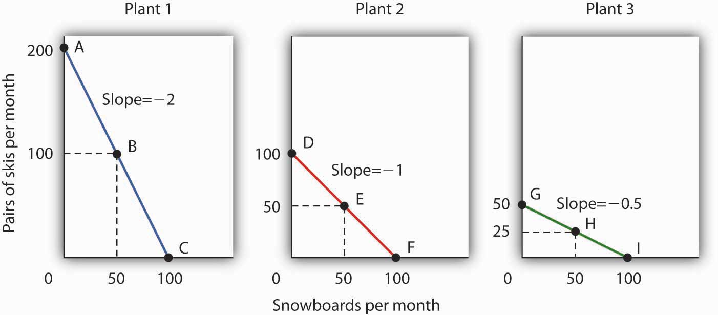 [Figure 3 - Production Possibilities at Three Plants]
The slopes of the production possibilities curves for each plant differ. The steeper the curve, the greater the opportunity cost of an additional snowboard. Here, the opportunity cost is lowest at Plant 3 and greatest at Plant 1.
The exhibit gives the slopes of the production possibilities curves for each of the firm’s three plants. The opportunity cost of an additional snowboard at each plant equals the absolute values of these slopes. More generally, the absolute value of the slope of any production possibilities curve at any point gives the opportunity cost of an additional unit of the good on the horizontal axis, measured in terms of the number of units of the good on the vertical axis that must be forgone.
The greater the absolute value of the slope of the production possibilities curve, the greater the opportunity cost will be. The plant for which the opportunity cost of an additional snowboard is greatest is the plant with the steepest production possibilities curve; the plant for which the opportunity cost is lowest is the plant with the flattest production possibilities curve. The plant with the lowest opportunity cost of producing snowboards is Plant 3; its slope of −0.5 means that Ms. Ryder must give up half a pair of skis in that plant to produce an additional snowboard. In Plant 2, she must give up one pair of skis to gain one more snowboard. We have already seen that an additional snowboard requires giving up two pairs of skis in Plant 1.
Comparative Advantage and the Production Possibilities Curve
To construct a combined production possibilities curve for all three plants, we can begin by asking how many pairs of skis Alpine Sports could produce if it were producing only skis. To find this quantity, we add up the values at the vertical intercepts of each of the production possibilities curves in [Figure 3 - Production Possibilities at Three Plants]. These intercepts tell us the maximum number of pairs of skis each plant can produce. Plant 1 can produce 200 pairs of skis per month, Plant 2 can produce 100 pairs of skis at per month, and Plant 3 can produce 50 pairs. Alpine Sports can thus produce 350 pairs of skis per month if it devotes its resources exclusively to ski production. In that case, it produces no snowboards.
Now suppose the firm decides to produce 100 snowboards. That will require shifting one of its plants out of ski production. Which one will it choose to shift? The sensible thing for it to do is to choose the plant in which snowboards have the lowest opportunity cost—Plant 3. It has an advantage not because it can produce more snowboards than the other plants (all the plants in this example are capable of producing up to 100 snowboards per month) but because it is the least productive plant for making skis. Producing a snowboard in Plant 3 requires giving up just half a pair of skis.
Economists say that an economy has a comparative advantage in producing a good or service if the opportunity cost of producing that good or service is lower for that economy than for any other. Plant 3 has a comparative advantage in snowboard production because it is the plant for which the opportunity cost of additional snowboards is lowest. To put this in terms of the production possibilities curve, Plant 3 has a comparative advantage in snowboard production (the good on the horizontal axis) because its production possibilities curve is the flattest of the three curves.
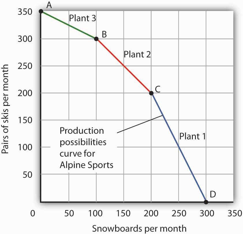 [Figure 4 - The Combined Production Possibilities Curve for Alpine Sports]
The curve shown combines the production possibilities curves for each plant. At point A, Alpine Sports produces 350 pairs of skis per month and no snowboards. If the firm wishes to increase snowboard production, it will first use Plant 3, which has a comparative advantage in snowboards.
Plant 3’s comparative advantage in snowboard production makes a crucial point about the nature of comparative advantage. It need not imply that a particular plant is especially good at an activity. In our example, all three plants are equally good at snowboard production. Plant 3, though, is the least efficient of the three in ski production. Alpine thus gives up fewer skis when it produces snowboards in Plant 3. Comparative advantage thus can stem from a lack of efficiency in the production of an alternative good rather than a special proficiency in the production of the first good.
The combined production possibilities curve for the firm’s three plants is shown in [Figure 4 - The Combined Production Possibilities Curve for Alpine Sports]. We begin at point A, with all three plants producing only skis. Production totals 350 pairs of skis per month and zero snowboards. If the firm were to produce 100 snowboards at Plant 3, ski production would fall by 50 pairs per month (recall that the opportunity cost per snowboard at Plant 3 is half a pair of skis). That would bring ski production to 300 pairs, at point B. If Alpine Sports were to produce still more snowboards in a single month, it would shift production to Plant 2, the facility with the next-lowest opportunity cost. Producing 100 snowboards at Plant 2 would leave Alpine Sports producing 200 snowboards and 200 pairs of skis per month, at point C. If the firm were to switch entirely to snowboard production, Plant 1 would be the last to switch because the cost of each snowboard there is 2 pairs of skis. With all three plants producing only snowboards, the firm is at point D on the combined production possibilities curve, producing 300 snowboards per month and no skis.
Notice that this production possibilities curve, which is made up of linear segments from each assembly plant, has a bowed-out shape; the absolute value of its slope increases as Alpine Sports produces more and more snowboards. This is a result of transferring resources from the production of one good to another according to comparative advantage. We shall examine the significance of the bowed-out shape of the curve in the next section.
The Law of Increasing Opportunity Cost
We see in [Figure 4 - The Combined Production Possibilities Curve for Alpine Sports] that, beginning at point A and producing only skis, Alpine Sports experiences higher and higher opportunity costs as it produces more snowboards. The fact that the opportunity cost of additional snowboards increases as the firm produces more of them is a reflection of an important economic law. The law of increasing opportunity cost holds that as an economy moves along its production possibilities curve in the direction of producing more of a particular good, the opportunity cost of additional units of that good will increase.
We have seen the law of increasing opportunity cost at work traveling from point A toward point D on the production possibilities curve in [Figure 4 - The Combined Production Possibilities Curve for Alpine Sports]. The opportunity cost of each of the first 100 snowboards equals half a pair of skis; each of the next 100 snowboards has an opportunity cost of 1 pair of skis, and each of the last 100 snowboards has an opportunity cost of 2 pairs of skis. The law also applies as the firm shifts from snowboards to skis. Suppose it begins at point D, producing 300 snowboards per month and no skis. It can shift to ski production at a relatively low cost at first. The opportunity cost of the first 200 pairs of skis is just 100 snowboards at Plant 1, a movement from point D to point C, or 0.5 snowboards per pair of skis. We would say that Plant 1 has a comparative advantage in ski production. The next 100 pairs of skis would be produced at Plant 2, where snowboard production would fall by 100 snowboards per month. The opportunity cost of skis at Plant 2 is 1 snowboard per pair of skis. Plant 3 would be the last plant converted to ski production. There, 50 pairs of skis could be produced per month at a cost of 100 snowboards, or an opportunity cost of 2 snowboards per pair of skis.
The bowed-out production possibilities curve for Alpine Sports illustrates the law of increasing opportunity cost. Scarcity implies that a production possibilities curve is downward sloping; the law of increasing opportunity cost implies that it will be bowed out, or concave, in shape.
The bowed-out curve of [Figure 4 - The Combined Production Possibilities Curve for Alpine Sports] becomes smoother as we include more production facilities. Suppose Alpine Sports expands to 10 plants, each with a linear production possibilities curve. Panel (a) of [Figure 5 - Production Possibilities for the Economy] shows the combined curve for the expanded firm, constructed as we did in [Figure 4 - The Combined Production Possibilities Curve for Alpine Sports]. This production possibilities curve includes 10 linear segments and is almost a smooth curve. As we include more and more production units, the curve will become smoother and smoother. In an actual economy, with a tremendous number of firms and workers, it is easy to see that the production possibilities curve will be smooth. We will generally draw production possibilities curves for the economy as smooth, bowed-out curves, like the one in Panel (b). This production possibilities curve shows an economy that produces only skis and snowboards. Notice the curve still has a bowed-out shape; it still has a negative slope. Notice also that this curve has no numbers. Economists often use models such as the production possibilities model with graphs that show the general shapes of curves but that do not include specific numbers.
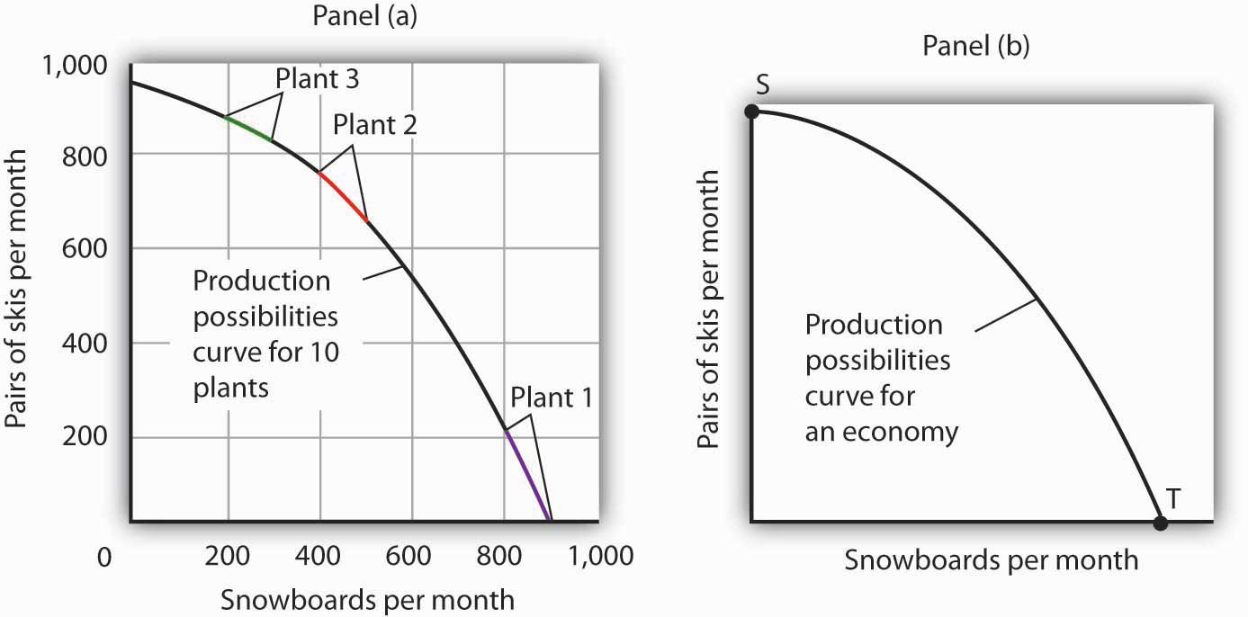
[Figure 5 - Production Possibilities for the Economy]
As we combine the production possibilities curves for more and more units, the curve becomes smoother. It retains its negative slope and bowed-out shape. In Panel (a) we have a combined production possibilities curve for Alpine Sports, assuming that it now has 10 plants producing skis and snowboards. Even though each of the plants has a linear curve, combining them according to comparative advantage, as we did with 3 plants in [Figure 4 - The Combined Production Possibilities Curve for Alpine Sports], produces what appears to be a smooth, nonlinear curve, even though it is made up of linear segments. In drawing production possibilities curves for the economy, we shall generally assume they are smooth and “bowed out,” as in Panel (b). This curve depicts an entire economy that produces only skis and snowboards.
Video: Production Possibilities
For another way of looking at the production possibilities curve, view the video below by economics teacher Jacob Clifford. He used the movie Monsters, Inc. to explain the production possibilities curve in an easier-to-understand way.

Answer the self check questions below to monitor your understanding of the concepts in this section.
Self Check Questions
- How would you construct a production possibilities curve?
- What is the comparative advantage in economy?
- Describe the law of opportunity cost.
- Name three points made in the video by Jacob Clifford.