
2.5: The Price System at Work
- Page ID
- 1689
\( \newcommand{\vecs}[1]{\overset { \scriptstyle \rightharpoonup} {\mathbf{#1}} } \)
\( \newcommand{\vecd}[1]{\overset{-\!-\!\rightharpoonup}{\vphantom{a}\smash {#1}}} \)
\( \newcommand{\id}{\mathrm{id}}\) \( \newcommand{\Span}{\mathrm{span}}\)
( \newcommand{\kernel}{\mathrm{null}\,}\) \( \newcommand{\range}{\mathrm{range}\,}\)
\( \newcommand{\RealPart}{\mathrm{Re}}\) \( \newcommand{\ImaginaryPart}{\mathrm{Im}}\)
\( \newcommand{\Argument}{\mathrm{Arg}}\) \( \newcommand{\norm}[1]{\| #1 \|}\)
\( \newcommand{\inner}[2]{\langle #1, #2 \rangle}\)
\( \newcommand{\Span}{\mathrm{span}}\)
\( \newcommand{\id}{\mathrm{id}}\)
\( \newcommand{\Span}{\mathrm{span}}\)
\( \newcommand{\kernel}{\mathrm{null}\,}\)
\( \newcommand{\range}{\mathrm{range}\,}\)
\( \newcommand{\RealPart}{\mathrm{Re}}\)
\( \newcommand{\ImaginaryPart}{\mathrm{Im}}\)
\( \newcommand{\Argument}{\mathrm{Arg}}\)
\( \newcommand{\norm}[1]{\| #1 \|}\)
\( \newcommand{\inner}[2]{\langle #1, #2 \rangle}\)
\( \newcommand{\Span}{\mathrm{span}}\) \( \newcommand{\AA}{\unicode[.8,0]{x212B}}\)
\( \newcommand{\vectorA}[1]{\vec{#1}} % arrow\)
\( \newcommand{\vectorAt}[1]{\vec{\text{#1}}} % arrow\)
\( \newcommand{\vectorB}[1]{\overset { \scriptstyle \rightharpoonup} {\mathbf{#1}} } \)
\( \newcommand{\vectorC}[1]{\textbf{#1}} \)
\( \newcommand{\vectorD}[1]{\overrightarrow{#1}} \)
\( \newcommand{\vectorDt}[1]{\overrightarrow{\text{#1}}} \)
\( \newcommand{\vectE}[1]{\overset{-\!-\!\rightharpoonup}{\vphantom{a}\smash{\mathbf {#1}}}} \)
\( \newcommand{\vecs}[1]{\overset { \scriptstyle \rightharpoonup} {\mathbf{#1}} } \)
\( \newcommand{\vecd}[1]{\overset{-\!-\!\rightharpoonup}{\vphantom{a}\smash {#1}}} \)
\(\newcommand{\avec}{\mathbf a}\) \(\newcommand{\bvec}{\mathbf b}\) \(\newcommand{\cvec}{\mathbf c}\) \(\newcommand{\dvec}{\mathbf d}\) \(\newcommand{\dtil}{\widetilde{\mathbf d}}\) \(\newcommand{\evec}{\mathbf e}\) \(\newcommand{\fvec}{\mathbf f}\) \(\newcommand{\nvec}{\mathbf n}\) \(\newcommand{\pvec}{\mathbf p}\) \(\newcommand{\qvec}{\mathbf q}\) \(\newcommand{\svec}{\mathbf s}\) \(\newcommand{\tvec}{\mathbf t}\) \(\newcommand{\uvec}{\mathbf u}\) \(\newcommand{\vvec}{\mathbf v}\) \(\newcommand{\wvec}{\mathbf w}\) \(\newcommand{\xvec}{\mathbf x}\) \(\newcommand{\yvec}{\mathbf y}\) \(\newcommand{\zvec}{\mathbf z}\) \(\newcommand{\rvec}{\mathbf r}\) \(\newcommand{\mvec}{\mathbf m}\) \(\newcommand{\zerovec}{\mathbf 0}\) \(\newcommand{\onevec}{\mathbf 1}\) \(\newcommand{\real}{\mathbb R}\) \(\newcommand{\twovec}[2]{\left[\begin{array}{r}#1 \\ #2 \end{array}\right]}\) \(\newcommand{\ctwovec}[2]{\left[\begin{array}{c}#1 \\ #2 \end{array}\right]}\) \(\newcommand{\threevec}[3]{\left[\begin{array}{r}#1 \\ #2 \\ #3 \end{array}\right]}\) \(\newcommand{\cthreevec}[3]{\left[\begin{array}{c}#1 \\ #2 \\ #3 \end{array}\right]}\) \(\newcommand{\fourvec}[4]{\left[\begin{array}{r}#1 \\ #2 \\ #3 \\ #4 \end{array}\right]}\) \(\newcommand{\cfourvec}[4]{\left[\begin{array}{c}#1 \\ #2 \\ #3 \\ #4 \end{array}\right]}\) \(\newcommand{\fivevec}[5]{\left[\begin{array}{r}#1 \\ #2 \\ #3 \\ #4 \\ #5 \\ \end{array}\right]}\) \(\newcommand{\cfivevec}[5]{\left[\begin{array}{c}#1 \\ #2 \\ #3 \\ #4 \\ #5 \\ \end{array}\right]}\) \(\newcommand{\mattwo}[4]{\left[\begin{array}{rr}#1 \amp #2 \\ #3 \amp #4 \\ \end{array}\right]}\) \(\newcommand{\laspan}[1]{\text{Span}\{#1\}}\) \(\newcommand{\bcal}{\cal B}\) \(\newcommand{\ccal}{\cal C}\) \(\newcommand{\scal}{\cal S}\) \(\newcommand{\wcal}{\cal W}\) \(\newcommand{\ecal}{\cal E}\) \(\newcommand{\coords}[2]{\left\{#1\right\}_{#2}}\) \(\newcommand{\gray}[1]{\color{gray}{#1}}\) \(\newcommand{\lgray}[1]{\color{lightgray}{#1}}\) \(\newcommand{\rank}{\operatorname{rank}}\) \(\newcommand{\row}{\text{Row}}\) \(\newcommand{\col}{\text{Col}}\) \(\renewcommand{\row}{\text{Row}}\) \(\newcommand{\nul}{\text{Nul}}\) \(\newcommand{\var}{\text{Var}}\) \(\newcommand{\corr}{\text{corr}}\) \(\newcommand{\len}[1]{\left|#1\right|}\) \(\newcommand{\bbar}{\overline{\bvec}}\) \(\newcommand{\bhat}{\widehat{\bvec}}\) \(\newcommand{\bperp}{\bvec^\perp}\) \(\newcommand{\xhat}{\widehat{\xvec}}\) \(\newcommand{\vhat}{\widehat{\vvec}}\) \(\newcommand{\uhat}{\widehat{\uvec}}\) \(\newcommand{\what}{\widehat{\wvec}}\) \(\newcommand{\Sighat}{\widehat{\Sigma}}\) \(\newcommand{\lt}{<}\) \(\newcommand{\gt}{>}\) \(\newcommand{\amp}{&}\) \(\definecolor{fillinmathshade}{gray}{0.9}\)The Price System at Work
Prices are considered to be neutral because they do not favor either the producer or the consumer. Prices are flexible when an unforeseen event, such as war, occurs. Prices will be adjusted to meet the unexpected situation and then over time, may return to previous levels. Prices are considered efficient because they are based on supply and demand; there is no need for a bureaucracy to create them. Finally, prices are easy to understand. From the time that we are old enough to buy something, we are familiar with how prices work in the market place.
Because of supply and demand in the free market economy, there are various prices that may prevail. A change in price in one market may affect the allocation of resources in that market, as well as between markets. We know this is how the market economy works because economists use economic models to help analyze behavior and predict outcomes. These types of models can help determine why there may be a surplus or a shortage in the market. In addition, economists use theories to help create what would be ideal conditions and outcomes, in order to measure the performance of the market or other types of economic systems.
Universal Generalizations
- Changes in supply and demand cause prices to change.
- The interaction between supply, demand, and price is illustrated by supply and demand graphs.
- The interaction between supply, demand, and non-price determinants is illustrated by supply and demand graphs.
- Economists use market models to predict how events impact possible changes in price.
Guiding Questions
- How are prices determined in a competitive market?
- How can economic models be used to predict and explain changes in price?
- Why is price elasticity important?
Video: Supply, Demand, Equilibrium, and Shifting Curves (Indiana Jones)
Equilibrium—Where Demand and Supply Intersect
Because the graphs for demand and supply curves both have price on the vertical axis and quantity on the horizontal axis, the demand curve and supply curve for a particular good or service can appear on the same graph. Together, demand and supply determine the price and the quantity that will be bought and sold in a market.
[Figure 1] illustrates the interaction of demand and supply in the market for gasoline. The demand curve (D), the supply curve (S), and [Table 1] contains the same information in tabular form.
Demand and Supply for Gasoline
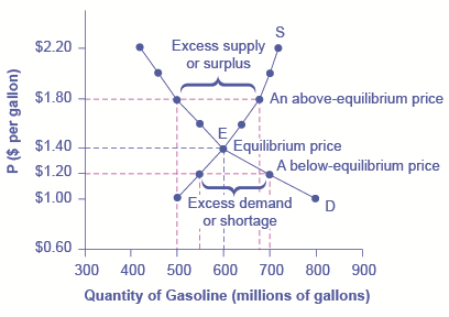
The demand curve (D) and the supply curve (S) intersect at the equilibrium point E, with a price of $1.40 and a quantity of 600. The equilibrium is the only price where quantity demanded is equal to quantity supplied. At a price above equilibrium like $1.80, quantity supplied exceeds the quantity demanded, so there is excess supply. At a price below equilibrium such as $1.20, quantity demanded exceeds quantity supplied, so there is excess demand.
| Price (per gallon) | Quantity demanded (millions of gallons) | Quantity supplied (millions of gallons) |
| $1.00 | 800 | 500 |
| $1.20 | 700 | 550 |
| $1.40 | 600 | 600 |
| $1.60 | 550 | 640 |
| $1.80 | 500 | 680 |
| $2.00 | 460 | 700 |
| $2.20 | 420 | 720 |
Remember this: When two lines on a diagram cross, this intersection usually means something. The point where the supply curve (S) and the demand curve (D) cross, designated by point E in [Figure 1], is called the equilibrium. The equilibrium price is the only price where the plans of consumers and the plans of producers agree—that is, where the amount of the product consumers want to buy (quantity demanded) is equal to the amount producers want to sell (quantity supplied). This common quantity is called the equilibrium quantity. At any other price, the quantity demanded does not equal the quantity supplied, so the market is not in equilibrium at that price.
In [Figure 1], the equilibrium price is $1.40 per gallon of gasoline and the equilibrium quantity is 600 million gallons. If you had only the demand and supply schedules, and not the graph, you could find the equilibrium by looking for the price level on the tables where the quantity demanded and the quantity supplied are equal.
The word “equilibrium” means “balance.” If a market is at its equilibrium price and quantity, then it has no reason to move away from that point. However, if a market is not at equilibrium, then economic pressures arise to move the market toward the equilibrium price and the equilibrium quantity.
Imagine, for example, that the price of a gallon of gasoline was above the equilibrium price—that is, instead of $1.40 per gallon, the price is $1.80 per gallon. This above-equilibrium price is illustrated by the dashed horizontal line at the price of $1.80 in [Figure 1]. At this higher price, the quantity demanded drops from 600 to 500. This decline in quantity reflects how consumers react to the higher price by finding ways to use less gasoline.
Additionally, at this higher price of $1.80, the quantity of gasoline supplied rises from the 600 to 680, as the higher price makes it more profitable for gasoline producers to expand their output. Now, consider how quantity demanded and quantity supplied are related at this above-equilibrium price. Quantity demanded has fallen to 500 gallons, while quantity supplied has risen to 680 gallons. In fact, at any above-equilibrium price, the quantity supplied exceeds the quantity demanded. We call this an excess supply or a surplus.
With a surplus, gasoline accumulates at gas stations, in tanker trucks, in pipelines, and at oil refineries. This accumulation puts pressure on gasoline sellers. If a surplus remains unsold, those firms involved in making and selling gasoline are not receiving enough cash to pay their workers and to cover their expenses. In this situation, some producers and sellers will want to cut prices, because it is better to sell at a lower price than not to sell at all. Once some sellers start cutting prices, others will follow to avoid losing sales. These price reductions in turn will stimulate a higher quantity demanded. So, if the price is above the equilibrium level, incentives built into the structure of demand and supply will create pressures for the price to fall toward the equilibrium.
Now suppose that the price is below its equilibrium level at $1.20 per gallon, as the dashed horizontal line at this price in [Figure 1] shows. At this lower price, the quantity demanded increases from 600 to 700 as drivers take longer trips, spend more minutes warming up the car in the driveway in wintertime, stop sharing rides to work, and buy larger cars that get fewer miles to the gallon. However, the below-equilibrium price reduces gasoline producers’ incentives to produce and sell gasoline, and the quantity supplied falls from 600 to 550.
When the price is below equilibrium, there is excess demand, or a shortage—that is, at the given price the quantity demanded, which has been stimulated by the lower price, now exceeds the quantity supplied, which had been depressed by the lower price. In this situation, eager gasoline buyers mob the gas stations, only to find many stations running short of fuel. Oil companies and gas stations recognize that they have an opportunity to make higher profits by selling what gasoline they have at a higher price. As a result, the price rises toward the equilibrium level.
Changes in Equilibrium Price and Quantity: The Four-Step Process
Let’s begin this discussion with a single economic event. It might be an event that affects demand, like a change in income, population, tastes, prices of substitutes or complements, or expectations about future prices. It might be an event that affects supply, like a change in natural conditions, input prices, or technology, or government policies that affect production. How does this economic event affect equilibrium price and quantity? We will analyze this question using a four-step process.
Step 1.
Draw a demand and supply model before the economic change took place. To establish the model requires four standard pieces of information: The law of demand, which tells us the slope of the demand curve; the law of supply, which gives us the slope of the supply curve; the shift variables for demand; and the shift variables for supply. From this model, find the initial equilibrium values for price and quantity.
Step 2.
Decide whether the economic change being analyzed affects demand or supply. In other words, does the event refer to something in the list of demand factors or supply factors?
Step 3.
Decide whether the effect on demand or supply causes the curve to shift to the right or to the left, and sketch the new demand or supply curve on the diagram. In other words, does the event increase or decrease the amount consumers want to buy or producers want to sell?
Step 4.
Identify the new equilibrium and then compare the original equilibrium price and quantity to the new equilibrium price and quantity.
Let’s consider one example that involves a shift in supply and one that involves a shift in demand. Then we will consider an example where both supply and demand shift.
In the summer of 2000, weather conditions were excellent for commercial salmon fishing off the California coast. Heavy rains meant higher than normal levels of water in the rivers, which helps the salmon to breed. Slightly cooler ocean temperatures stimulated the growth of plankton, the microscopic organisms at the bottom of the ocean food chain, providing everything in the ocean with a hearty food supply. The ocean stayed calm during fishing season, so commercial fishing operations did not lose many days to bad weather. How did these climate conditions affect the quantity and price of salmon?
[Figure 2] illustrates the four-step approach, which is explained below, to work through this problem. [Table 2] provides the information to work the problem as well.
Good Weather for Salmon Fishing: The Four-Step Process
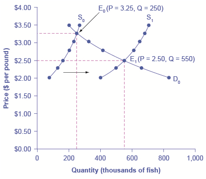
Unusually good weather leads to changes in the price and quantity of salmon.
| Price per Pound | Quantity Supplied in 1999 | Quantity Supplied in 2000 | Quantity Demanded |
| $2.00 | 80 | 400 | 840 |
| $2.25 | 120 | 480 | 680 |
| $2.50 | 160 | 550 | 550 |
| $2.75 | 200 | 600 | 450 |
| $3.00 | 230 | 640 | 350 |
| $3.25 | 250 | 670 | 250 |
| $3.50 | 270 | 700 | 200 |
Step 1. Draw a demand and supply model to illustrate the market for salmon in the year before the good weather conditions began. The demand curve D0 and the supply curve S0 show that the original equilibrium price is $3.25 per pound and the original equilibrium quantity is 250,000 fish. (This price per pound is what commercial buyers pay at the fishing docks; what consumers pay at the grocery is higher.)
Step 2. Did the economic event affect supply or demand? Good weather is an example of a natural condition that affects supply.
Step 3. Was the effect on supply an increase or a decrease? Good weather is a change in natural conditions that increases the quantity supplied at any given price. The supply curve shifts to the right, moving from the original supply curve S0 to the new supply curve S1, which is shown in both the table and the figure.
Step 4. Compare the new equilibrium price and quantity to the original equilibrium. At the new equilibrium E1, the equilibrium price falls from $3.25 to $2.50, but the equilibrium quantity increases from 250,000 to 550,000 salmon. Notice that the equilibrium quantity demanded increased, even though the demand curve did not move.
In short, good weather conditions increased supply of the California commercial salmon. The result was a higher equilibrium quantity of salmon bought and sold in the market at a lower price.
According to the Pew Research Center for People and the Press, more and more people, especially younger people, are getting their news from online and digital sources. The majority of U.S. adults now own smartphones or tablets, and most of those Americans say they use them in part to get the news. From 2004 to 2012, the share of Americans who reported getting their news from digital sources increased from 24% to 39%. How has this affected consumption of print news media, and radio and television news? [Figure 3] and the text below illustrates using the four-step analysis to answer this question.
The Print News Market: A Four-Step Analysis
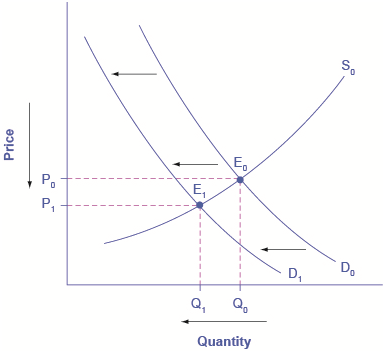
A change in tastes from print news sources to digital sources results in a leftward shift in demand for the former. The result is a decrease in both equilibrium price and quantity.
Step 1. Develop a demand and supply model to think about what the market looked like before the event. The demand curve D0 and the supply curve S0 show the original relationships. In this case, the analysis is performed without specific numbers on the price and quantity axis.
Step 2. Did the change described affect supply or demand? A change in tastes, from traditional news sources (print, radio, and television) to digital sources, caused a change in demand for the former.
Step 3. Was the effect on demand positive or negative? A shift to digital news sources will tend to mean a lower quantity demanded of traditional news sources at every given price, causing the demand curve for print and other traditional news sources to shift to the left, from D0 to D1.
Step 4. Compare the new equilibrium price and quantity to the original equilibrium price. The new equilibrium (E1) occurs at a lower quantity and a lower price than the original equilibrium (E0).
The decline in print news reading predates 2004. Print newspaper circulation peaked in 1973 and has declined since then due to competition from television and radio news. In 1991, 55% of Americans indicated they got their news from print sources, while only 29% did so in 2012. Radio news has followed a similar path in recent decades, with the share of Americans getting their news from radio declining from 54% in 1991 to 33% in 2012. Television news has held its own over the last 15 years, with a market share staying in the mid to upper fifties. What does this suggest for the future, given that two-thirds of Americans under 30 years old say they do not get their news from television at all?
A Combined Example
The U.S. Postal Service is facing difficult challenges. Compensation for postal workers tends to increase most years due to cost-of-living increases. At the same time, more and more people are using email, text, and other digital message forms such as Facebook and Twitter to communicate with friends and others. What does this suggest about the continued viability of the Postal Service? [Figure 4] and the text below illustrates using the four-step analysis to answer this question.
Higher Compensation for Postal Workers: A Four-Step Analysis
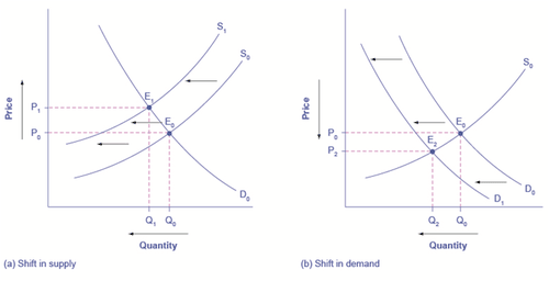
(a) Higher labor compensation causes a leftward shift in the supply curve, a decrease in the equilibrium quantity, and an increase in the equilibrium price. (b) A change in tastes away from Postal Services causes a leftward shift in the demand curve, a decrease in the equilibrium quantity, and a decrease in the equilibrium price.
Since this problem involves two disturbances, we need two four-step analyses, the first to analyze the effects of higher compensation for postal workers, the second to analyze the effects of many people switching from “snail mail” to email and other digital messages.
Since this problem involves two disturbances, we need two four-step analyses, the first to analyze the effects of higher compensation for postal workers, the second to analyze the effects of many people switching from “snail mail” to email and other digital messages.
[Figure 4 (a)] shows the shift in supply discussed in the following steps.
Step 1. Draw a demand and supply model to illustrate what the market for the U.S. Postal Service looked like before this scenario starts. The demand curve D0 and the supply curve S0 show the original relationships.
Step 2. Did the change described affect supply or demand? Labor compensation is a cost of production. A change in production costs caused a change in supply for the Postal Service.
Step 3. Was the effect on supply positive or negative? Higher labor compensation leads to a lower quantity supplied of traditional news sources at every given price, causing the supply curve for print and other traditional news sources to shift to the left, from S0 to S1.
Step 4. Compare the new equilibrium price and quantity to the original equilibrium price. The new equilibrium (E1) occurs at a lower quantity and a higher price than the original equilibrium (E0).
[Figure 4 (b)] shows the shift in demand discussed in the following steps.
Step 1. Draw a demand and supply model to illustrate what the market for U.S. Postal Services looked like before this scenario starts. The demand curve D0 and the supply curve S0 show the original relationships. Note that this diagram is independent of the diagram in panel (a).
Step 2. Did the change described affect supply or demand? A change in tastes away from snail mail toward digital messages will cause a change in demand for the Postal Service.
Step 3. Was the effect on supply positive or negative? A change in tastes away from snail mail toward digital messages leads to a lower quantity demanded of Postal Services at every given price, causing the demand curve for Postal Services to shift to the left, from D0 to D1.
Step 4. Compare the new equilibrium price and quantity to the original equilibrium price. The new equilibrium (E2) occurs at a lower quantity and a lower price than the original equilibrium (E0).
The final step in a scenario where both supply and demand shift is to combine the two individual analyses to determine what happens to the equilibrium quantity and price. Graphically, we superimpose the previous two diagrams one on top of the other, as in [Figure 5].
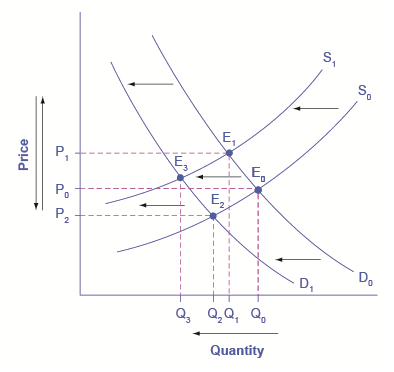 Supply and demand shifts cause changes in equilibrium price and quantity.
Results:
Effect on Quantity:
The effect of higher labor compensation on Postal Services because it raises the cost of production is to decrease the equilibrium quantity. The effect of a change in tastes away from snail mail is to decrease the equilibrium quantity. Since both shifts are to the left, the overall impact is a decrease in the equilibrium quantity of Postal Services (Q3). This is easy to see graphically, since Q3 is to the left of Q0.
Effect on Price:
The overall effect on price is more complicated. The effect of higher labor compensation on Postal Services, because it raises the cost of production, is to increase the equilibrium price. The effect of a change in tastes away from snailmail is to decrease the equilibrium price. Since the two effects are in opposite directions, unless we know the magnitudes of the two effects, the overall effect is unclear. This is not unusual. When both curves shift, typically we can determine the overall effect on price or on quantity, but not on both. In this case, we determined the overall effect on the equilibrium quantity, but not on the equilibrium price. In other cases, it might be the opposite.
What is the difference between shifts of demand or supply versus movements along a demand or supply curve?
One common mistake in applying the demand and supply framework is to confuse the shift of a demand or a supply curve with movement along a demand or supply curve. As an example, consider a problem that asks whether a drought will increase or decrease the equilibrium quantity and equilibrium price of wheat. Lee, a student in an introductory economics class, might reason:
“Well, it is clear that a drought reduces supply, so I will shift back the supply curve, as in the shift from the original supply curve S0 to S1 shown on the diagram (called Shift 1). So the equilibrium moves from E0 to E1, the equilibrium quantity is lower and the equilibrium price is higher. Then, a higher price makes farmers more likely to supply the good, so the supply curve shifts right, as shown by the shift from S1 to S2, on the diagram (shown as Shift 2), so that the equilibrium now moves from E1 to E2. The higher price, however, also reduces demand and so causes demand to shift back, like the shift from the original demand curve, D0 to D1 on the diagram (labeled Shift 3), and the equilibrium moves from E2 to E3.”
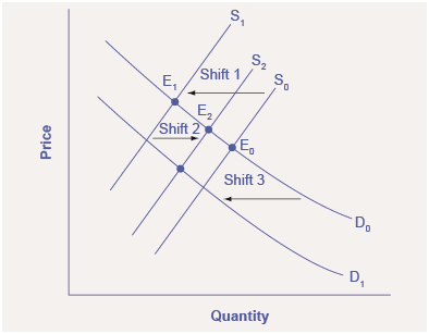
A shift in one curve never causes a shift in the other curve. Rather, a shift in one curve causes a movement along the second curve.
At about this point, Lee suspects that this answer is headed down the wrong path. Think about what might be wrong with Lee’s logic, and then read the answer that follows.
Answer: Lee’s first step is correct: that is, drought shifts back the supply curve of wheat and leads to a prediction of a lower equilibrium quantity and a higher equilibrium price. This corresponds to a movement along the original demand curve (D0), from E0 to E1. The rest of Lee’s argument is wrong, because it mixes up shifts in supply with quantity supplied, and shifts in demand with quantity demanded. A higher or lower price never shifts the supply curve, as suggested by the shift in supply from S1 to S2. Instead, a price change leads to a movement along a given supply curve. Similarly, a higher or lower price never shifts a demand curve, as suggested in the shift from D0 to D1. Instead, a price change leads to a movement along a given demand curve. Remember, a change in the price of a good never causes the demand or supply curve for that good to shift.
Think carefully about the timeline of events: What happens first, what happens next? What is the cause, what is the effect? If you keep the order right, you are more likely to get the analysis correct.
In the four-step analysis of how economic events affect equilibrium price and quantity, the movement from the old to the new equilibrium seems immediate. As a practical matter, however, prices and quantities often do not zoom straight to equilibrium. More realistically, when an economic event causes demand or supply to shift, prices and quantities set off in the general direction of equilibrium. Indeed, even as they are moving toward one new equilibrium, prices are often then pushed by another change in demand or supply toward another equilibrium.
Demand, Supply, and Efficiency
The familiar demand and supply diagram holds within it the concept of economic efficiency. One typical way that economists define efficiency is when it is impossible to improve the situation of one party without imposing a cost on another. Conversely, if a situation is inefficient, it becomes possible to benefit at least one party without imposing costs on others.
Efficiency in the demand and supply model has the same basic meaning: The economy is getting as much benefit as possible from its scarce resources and all the possible gains from trade have been achieved. In other words, the optimal amount of each good and service is being produced and consumed.
The economists often use the economic model to help analyze behavior and predict outcomes. These models are often represented with supply and demand curves in order to example the concept of market equilibrium to show how prices are relatively stable and the quantity of output supplies is equal to the quantity demanded. Prices in a competitive market are established by supply and demand. If prices are too high there will be a surplus. If prices are too low there will be a shortage. Eventually the market will correct itself so that it reaches market equilibrium and there will be neither a surplus nor a shortage.
Prices will change in response to a change in supply or a change in demand. What economists have determined is that the size of the price changes are affected by "elasticity". Price elasticity can influence consumers. An item that is a luxury may be demand more if the product goes on sale, however, if the product is a need then the change in price does not usually influence consumer demand.
Of course the theory of competitive pricing is just that, a theory. It represents a set of ideal conditions and outcomes and is another model that allows economists to measure the performance of less competitive markets.
Read this article that addresses how the 2012 drought impacted food prices:
Why Are Food Prices Rising - Understanding the Effect of Droughts
 Answer the self check questions below to monitor your understanding of the concepts in this section.
Self Check Questions
- What is an economic model?
- What is market equilibrium?
- How does the market find its equilibrium?
- What is a surplus? Why does it occur?
- What is a shortage? Why does it occur?
- What is equilibrium price?
- Why do economists use models?
- What is the theory of competitive pricing?