2.2.2: Graphs of Polynomials Using Zeros

Graphs of Polynomials Using Zeros

How is finding and using the zeroes of a higher-degree polynomial related to the same process you have used in the past on quadratic functions?

---

Graphing Polynomials Using Zeros

The following procedure can be followed when graphing a polynomial function.

• Use the leading-term test to determine the end behavior of the graph.
• Find the x−intercept(s) of f(x) by setting f(x)=0 and then solving for x.
• Find the y−intercept of f(x) by setting y=f(0) and finding y.
• Use the x−intercept(s) to divide the x−axis into intervals and then choose test points to determine the sign of f(x) on each interval.
• Plot the test points.
• If necessary, find additional points to determine the general shape of the graph.

The Leading-Term Test

If a_nxⁿ is the leading term of a polynomial. Then the behavior of the graph as x→∞ or x→−∞ can be known by one the four following behaviors:

2. If a_n<0 and n even: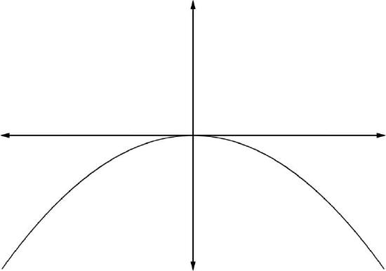

3. If a_n>0 and n odd: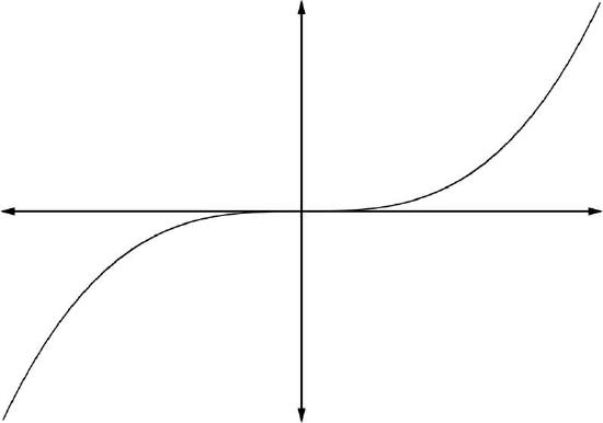

4. If a_n<0 and n odd: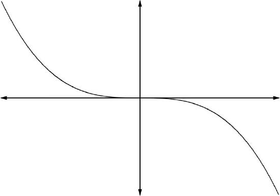

---

Examples

Example 1

Earlier, you were asked to identify some similarities in graphing using zeroes between quadratic functions and higher-degree polynomials.

Solution

Despite the more complex nature of the graphs of higher-degree polynomials, the general process of graphing using zeroes is actually very similar. In both cases, your goal is to locate the points where the graph crosses the x or y axis. In both cases, this is done by setting the y value equal to zero and solving for x to find the x axis intercepts, and setting the x value equal to zero and solving for y to find the y axis intercepts.

Example 2

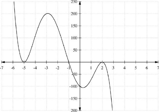
Find the roots (zeroes) of the polynomial:

h(x)=x³+2x²−5x−6

Solution

Start by factoring:

h(x)=x³+2x²−5x−6=(x+1)(x−2)(x+3)

To find the zeros, set h(x)=0 and solve for x.

(x+1)(x−2)(x+3)=0

This gives

x+1=0

x−2=0

x+3=0

or

x=-1

x=2

x=-3

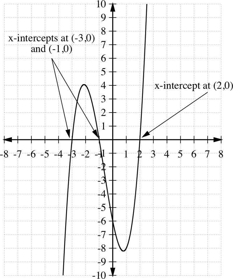
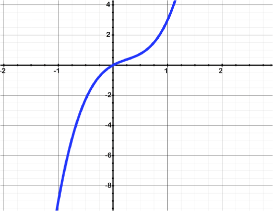
So we say that the solution set is {−3,−1,2}. They are the zeros of the function h(x). The zeros of h(x) are the x−intercepts of the graph y=h(x) below.

Example 3

Find the zeros of g(x)=−(x−2)(x−2)(x+1)(x+5)(x+5)(x+5).

Solution

The polynomial can be written as

g(x)=−(x−2)²(x+1)(x+5)³

To solve the equation, we simply set it equal to zero

−(x−2)²(x+1)(x+5)³=0

this gives

x−2=0

x+1=0

x+5=0

or

x=2

x=-1

x=-5

Notice the occurrence of the zeros in the function. The factor (x−2) occurred twice (because it was squared), the factor (x+1) occurred once and the factor (x+5) occurred three times. We say that the zero we obtain from the factor (x−2) has a multiplicity k=2 and the factor (x+5) has a multiplicity k=3.

Example 4

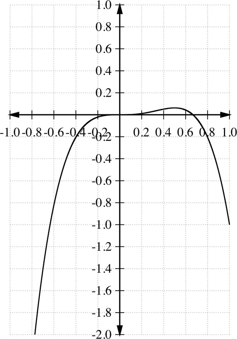
Graph the polynomial function f(x)=−3x⁴+2x³.

Solution

Since the leading term here is −3x⁴ then a_n=−3<0, and n=4 even. Thus the end behavior of the graph as x→∞ and x→−∞ is that of Box #2, item 2.

We can find the zeros of the function by simply setting f(x)=0 and then solving for x.

−3x⁴+2x³=0

−x³(3x−2)=0

This gives

x=0 or x=\(\ 2\over 3\)

So we have two x−intercepts, at x=0 and at x=\(\ 2\over 3\), with multiplicity k=3 for x=0 and multiplicity k=1 for x=\(\ 2\over 3\)

To find the y−intercept, we find f(0), which gives

f(0)=0

So the graph passes the y−axis at y=0.

Since the x−intercepts are 0 and \(\ 2\over 3\), they divide the x−axis into three intervals: (−∞, 0), (0, \(\ 2\over 3\)), and (\(\ 2\over 3\), ∞). Now we are interested in determining at which intervals the function f(x) is negative and at which intervals it is positive. To do so, we construct a table and choose a test value for x from each interval and find the corresponding f(x) at that value.

Interval	Test Value x	f(x)	Sign of f(x)	Location of points on the graph
(−∞, 0)	-1	-5	-	below the x−axis
(0, \(\ 2\over 3\))	\(\ 1\over 2\)	\(\ 1\over 16\)	+	above the x−axis
(\(\ 2\over 3\), ∞)	1	-1	-	below the x−axis

Those test points give us three additional points to plot: (−1, −5), (\(\ 1\over 2\), \(\ 1\over 16\)), and (1, -1). Now we are ready to plot our graph. We have a total of three intercept points, in addition to the three test points. We also know how the graph is behaving as x→−∞ and x→+∞. This information is usually enough to make a rough sketch of the graph. If we need additional points, we can simply select more points to complete the graph.

Example 5

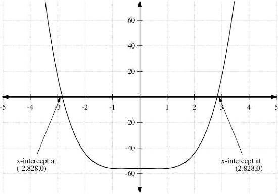
Find the zeros and sketch a graph of the polynomial

f(x)=x⁴−x²−56

Solution

This is a factorable equation,

f(x)=x⁴−x²−56

=(x²−8)(x²+7)

Setting f(x)=0,

(x²−8)(x²+7)=0

the first term gives

x²−8=0

x²=0

x= ±\(\ \sqrt{8}\)

= ±\(\ 2\sqrt{2}\)

and the second term gives

x²+7=0

x²=−7

x=±\(\ \sqrt{-7}\)

=±\(\ i\sqrt{7}\)

So the solutions are ±\(\ 2\sqrt{2}\) and ±\(\ i\sqrt{7}\), a total of four zeros of f(x). Keep in mind that only the real zeros of a function correspond to the x−intercept of its graph.

Example 6

Graph g(x)=−(x−2)²(x+1)(x+5)³.

Solution

Use the zeros to create a table of intervals and see whether the function is above or below the x−axis in each interval:

Interval	Test value x	g(x)	Sign of g(x)	Location of graph relative to x−axis
(−∞, −5)	-6	320	+	Above
x=−5	-5	0	NA
(-5, -1)	-2	144	+	Above
x=−1	-1	0	NA
(-1, 2)	0	-100	-	Below
x=2	2	0	NA
(2, ∞)	3	-256	-	Below

Finally, use this information and the test points to sketch a graph of g(x).

---

Review

1. If c is a zero of f, then c is a/an _________________________ of the graph of f.
2. If c is a zero of f, then (x - c) is a factor of ___________________?
3. Find the zeros of the polynomial: P(x)=x³−5x²+6x

Consider the function: f(x)=−3(x−3)⁴(5x−2)(2x−1)³(4−x)².

4. How many zeros (x-intercepts) are there?
5. What is the leading term?

Find the zeros and graph the polynomial. Be sure to label the x-intercepts, y-intercept (if possible) and have correct end behavior. You may use technology for questions 9-12.

6. P(x)=−2(x+1)²(x−3)
7. P(x)=x³+3x²−4x−12
8. f(x)=−2x³+6x²+9x+6
9. f(x)=−4x²−7x+3
10. f(x)=2x⁵+4x³+8x²+6x
11. f(x)=x⁴−3x²
12. g(x)=x²−|x|
13. Given: P(x)=(3x+2)(x−7)²(9x+2)³

State:

1. The leading term:
2. The degree of the polynomial:
3. The leading coefficient:

Determine the equation of the polynomial based on the graph:

14. 

15. 

---

Review (Answers)

To see the Review answers, open this PDF file and look for section 2.4.

---

Vocabulary

Term	Definition
Cubic Function	A cubic function is a function containing an x^3 term as the highest power of x.
Intercept	The intercepts of a curve are the locations where the curve intersects the x and y axes. An x intercept is a point at which the curve intersects the x-axis. A y intercept is a point at which the curve intersects the y-axis.
interval	An interval is a specific and limited part of a function.
Leading-Term Test	The leading-term test is a test to determine the end behavior of a polynomial function.
Polynomial	A polynomial is an expression with at least one algebraic term, but which does not indicate division by a variable or contain variables with fractional exponents.
Polynomial Graph	A polynomial graph is the graph of a polynomial function. The term is most commonly used for polynomial functions with a degree of at least three.
Quartic Function	A quartic function is a function f(x) containing an x^4 term as the highest power of ''x''.
Roots	The roots of a function are the values of x that make y equal to zero.
Zeroes	The zeroes of a function f(x) are the values of x that cause f(x) to be equal to zero.