2.3.1: Graphs of Basic Rational Functions
- Page ID
- 14196
\( \newcommand{\vecs}[1]{\overset { \scriptstyle \rightharpoonup} {\mathbf{#1}} } \)
\( \newcommand{\vecd}[1]{\overset{-\!-\!\rightharpoonup}{\vphantom{a}\smash {#1}}} \)
\( \newcommand{\dsum}{\displaystyle\sum\limits} \)
\( \newcommand{\dint}{\displaystyle\int\limits} \)
\( \newcommand{\dlim}{\displaystyle\lim\limits} \)
\( \newcommand{\id}{\mathrm{id}}\) \( \newcommand{\Span}{\mathrm{span}}\)
( \newcommand{\kernel}{\mathrm{null}\,}\) \( \newcommand{\range}{\mathrm{range}\,}\)
\( \newcommand{\RealPart}{\mathrm{Re}}\) \( \newcommand{\ImaginaryPart}{\mathrm{Im}}\)
\( \newcommand{\Argument}{\mathrm{Arg}}\) \( \newcommand{\norm}[1]{\| #1 \|}\)
\( \newcommand{\inner}[2]{\langle #1, #2 \rangle}\)
\( \newcommand{\Span}{\mathrm{span}}\)
\( \newcommand{\id}{\mathrm{id}}\)
\( \newcommand{\Span}{\mathrm{span}}\)
\( \newcommand{\kernel}{\mathrm{null}\,}\)
\( \newcommand{\range}{\mathrm{range}\,}\)
\( \newcommand{\RealPart}{\mathrm{Re}}\)
\( \newcommand{\ImaginaryPart}{\mathrm{Im}}\)
\( \newcommand{\Argument}{\mathrm{Arg}}\)
\( \newcommand{\norm}[1]{\| #1 \|}\)
\( \newcommand{\inner}[2]{\langle #1, #2 \rangle}\)
\( \newcommand{\Span}{\mathrm{span}}\) \( \newcommand{\AA}{\unicode[.8,0]{x212B}}\)
\( \newcommand{\vectorA}[1]{\vec{#1}} % arrow\)
\( \newcommand{\vectorAt}[1]{\vec{\text{#1}}} % arrow\)
\( \newcommand{\vectorB}[1]{\overset { \scriptstyle \rightharpoonup} {\mathbf{#1}} } \)
\( \newcommand{\vectorC}[1]{\textbf{#1}} \)
\( \newcommand{\vectorD}[1]{\overrightarrow{#1}} \)
\( \newcommand{\vectorDt}[1]{\overrightarrow{\text{#1}}} \)
\( \newcommand{\vectE}[1]{\overset{-\!-\!\rightharpoonup}{\vphantom{a}\smash{\mathbf {#1}}}} \)
\( \newcommand{\vecs}[1]{\overset { \scriptstyle \rightharpoonup} {\mathbf{#1}} } \)
\(\newcommand{\longvect}{\overrightarrow}\)
\( \newcommand{\vecd}[1]{\overset{-\!-\!\rightharpoonup}{\vphantom{a}\smash {#1}}} \)
\(\newcommand{\avec}{\mathbf a}\) \(\newcommand{\bvec}{\mathbf b}\) \(\newcommand{\cvec}{\mathbf c}\) \(\newcommand{\dvec}{\mathbf d}\) \(\newcommand{\dtil}{\widetilde{\mathbf d}}\) \(\newcommand{\evec}{\mathbf e}\) \(\newcommand{\fvec}{\mathbf f}\) \(\newcommand{\nvec}{\mathbf n}\) \(\newcommand{\pvec}{\mathbf p}\) \(\newcommand{\qvec}{\mathbf q}\) \(\newcommand{\svec}{\mathbf s}\) \(\newcommand{\tvec}{\mathbf t}\) \(\newcommand{\uvec}{\mathbf u}\) \(\newcommand{\vvec}{\mathbf v}\) \(\newcommand{\wvec}{\mathbf w}\) \(\newcommand{\xvec}{\mathbf x}\) \(\newcommand{\yvec}{\mathbf y}\) \(\newcommand{\zvec}{\mathbf z}\) \(\newcommand{\rvec}{\mathbf r}\) \(\newcommand{\mvec}{\mathbf m}\) \(\newcommand{\zerovec}{\mathbf 0}\) \(\newcommand{\onevec}{\mathbf 1}\) \(\newcommand{\real}{\mathbb R}\) \(\newcommand{\twovec}[2]{\left[\begin{array}{r}#1 \\ #2 \end{array}\right]}\) \(\newcommand{\ctwovec}[2]{\left[\begin{array}{c}#1 \\ #2 \end{array}\right]}\) \(\newcommand{\threevec}[3]{\left[\begin{array}{r}#1 \\ #2 \\ #3 \end{array}\right]}\) \(\newcommand{\cthreevec}[3]{\left[\begin{array}{c}#1 \\ #2 \\ #3 \end{array}\right]}\) \(\newcommand{\fourvec}[4]{\left[\begin{array}{r}#1 \\ #2 \\ #3 \\ #4 \end{array}\right]}\) \(\newcommand{\cfourvec}[4]{\left[\begin{array}{c}#1 \\ #2 \\ #3 \\ #4 \end{array}\right]}\) \(\newcommand{\fivevec}[5]{\left[\begin{array}{r}#1 \\ #2 \\ #3 \\ #4 \\ #5 \\ \end{array}\right]}\) \(\newcommand{\cfivevec}[5]{\left[\begin{array}{c}#1 \\ #2 \\ #3 \\ #4 \\ #5 \\ \end{array}\right]}\) \(\newcommand{\mattwo}[4]{\left[\begin{array}{rr}#1 \amp #2 \\ #3 \amp #4 \\ \end{array}\right]}\) \(\newcommand{\laspan}[1]{\text{Span}\{#1\}}\) \(\newcommand{\bcal}{\cal B}\) \(\newcommand{\ccal}{\cal C}\) \(\newcommand{\scal}{\cal S}\) \(\newcommand{\wcal}{\cal W}\) \(\newcommand{\ecal}{\cal E}\) \(\newcommand{\coords}[2]{\left\{#1\right\}_{#2}}\) \(\newcommand{\gray}[1]{\color{gray}{#1}}\) \(\newcommand{\lgray}[1]{\color{lightgray}{#1}}\) \(\newcommand{\rank}{\operatorname{rank}}\) \(\newcommand{\row}{\text{Row}}\) \(\newcommand{\col}{\text{Col}}\) \(\renewcommand{\row}{\text{Row}}\) \(\newcommand{\nul}{\text{Nul}}\) \(\newcommand{\var}{\text{Var}}\) \(\newcommand{\corr}{\text{corr}}\) \(\newcommand{\len}[1]{\left|#1\right|}\) \(\newcommand{\bbar}{\overline{\bvec}}\) \(\newcommand{\bhat}{\widehat{\bvec}}\) \(\newcommand{\bperp}{\bvec^\perp}\) \(\newcommand{\xhat}{\widehat{\xvec}}\) \(\newcommand{\vhat}{\widehat{\vvec}}\) \(\newcommand{\uhat}{\widehat{\uvec}}\) \(\newcommand{\what}{\widehat{\wvec}}\) \(\newcommand{\Sighat}{\widehat{\Sigma}}\) \(\newcommand{\lt}{<}\) \(\newcommand{\gt}{>}\) \(\newcommand{\amp}{&}\) \(\definecolor{fillinmathshade}{gray}{0.9}\)Graphing Rational Functions in Standard Form
The standard form of a rational function is given by the equation \(\ f(x)=\frac{a}{x-h}+k\). What are the asymptotes of this equation?
Rational Function
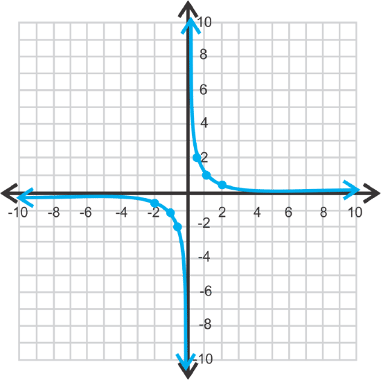
A rational function is in the form \(\ \frac{p(x)}{q(x)}\) where \(\ p(x)\) are polynomials and \(\ q(x)\)≠0. The parent graph for rational functions is \(\ y= \frac{1}{x}\), and the shape is called a hyperbola.
| \(\ x\) | \(\ y\) |
|---|---|
| −4 | \(\ -\frac{1}{4}\) |
| −2 | \(\ -\frac{1}{2}\) |
| −1 | −1 |
| \(\ -\frac{1}{2}\) | −2 |
| \(\ \frac{1}{2}\) | 2 |
| 1 | 1 |
| 2 | \(\ \frac{1}{2}\) |
| 4 | \(\ \frac{1}{4}\) |
 [Figure1]
Notice the following properties of this hyperbola: the x-axis is a horizontal asymptote, the y-axis is a vertical asymptote, and the domain and range are all real numbers except where the asymptotes are. Recall that the vertical asymptote is the value that makes the denominator zero because we cannot divide by zero. For the horizontal asymptote, it is the value where the range is not defined.
The two parts of the graph are called branches. In the case with a hyperbola, the branches are always symmetrical about the point where the asymptotes intersect. In this example, they are symmetrical about the origin.
In this lesson, all the rational functions will have the form \(\ f(x)=\frac{a}{x-h}+k\)
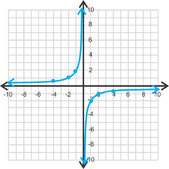
Let's graph \(\ f(x)=\frac{-2}{x}\) and find any asymptotes, the domain, range, and any zeros.
Let’s make a table of values.
| \(\ x\) | \(\ y\) |
|---|---|
| 1 | −2 |
| 2 | −1 |
| 4 | \(\ -\frac{1}{2}\) |
Notice that these branches are in the second and fourth quadrants. This is because of the negative sign in front of the 2, or \(\ a\). The horizontal and vertical asymptotes are still the \(\ x\) and \(\ y\)-axes. There are no zeros, or \(\ x\)-intercepts, because the \(\ x\)-axis is an asymptote. The domain and range are all non-zero real numbers (all real numbers except zero).
 [Figure2]
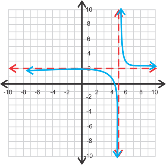
Now, let's graph \(\ y=\frac{1}{x-5}+2\) and find all asymptotes, zeros, the domain and range.
For \(\ y=\frac{1}{x-5}+2\), the vertical asymptote is x=5 because that would make the denominator zero and we cannot divide by zero. When x=5, the value of the function would be \(\ y=\frac{1}{0}+2\), making the range undefined at \(\ y=2\). The shape and location of the branches are the same as the parent graph, just shifted to the right 5 units and up 2 units.
 [Figure3]
Therefore, for the general form of a rational function, \(\ y=\frac{a}{x-h}+k, x=h\) is the vertical asymptote and \(\ y=k\) is the horizontal asymptote.
The domain is all real numbers; \(\ x\)≠5 and the range is all real numbers; \(\ y\)≠2. To find the zero, set the function equal to zero and solve for \(\ x\).
\(\ \begin{aligned}
0 &=\frac{1}{x-5}+2 \\
-2 &=\frac{1}{x-5} \\
-2 x+10 &=1 \\
-2 x &=-9 \\
x &=\frac{9}{2}=4.5
\end{aligned}\)
To find the y-intercept, set x=0, and solve for y. \(\ y=\frac{1}{0-5}+2=-\frac{1}{5}+2=1 \frac{4}{5}\).
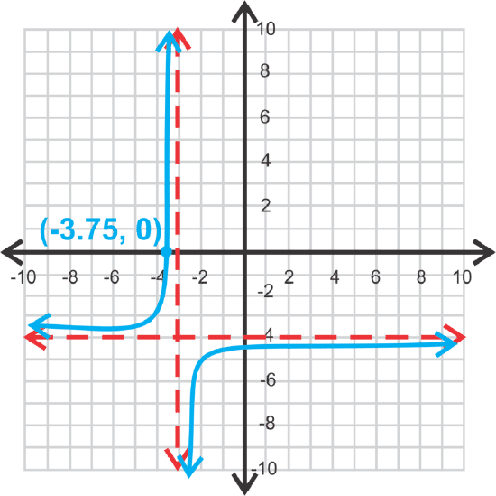
Finally, let's find the equation of the hyperbola below.
We know that the numerator will be negative because the branches of this hyperbola are in the second and fourth quadrants. The asymptotes are x=−3 and y=−4. So far, we know \(\ y=\frac{a}{x+3}-4\). In order to determine \(\ a\), we can use the given x-intercept.
 [Figure4]
\(\ \begin{aligned}
0&=\frac{a}{-3.75+3}-4\\
4 &=\frac{a}{-0.75} \quad\quad\quad\quad \text { The equation is } y=\frac{-3}{x+3}-4\\
-3 &=a
\end{aligned}\)
Examples
Earlier, you were asked to find the asymptotes of the equation \(\ f(x)=\frac{a}{x-h}+k\).
Solution
From the previous problems, we've seen that the vertical asymptote occurs when the denominator of the equation equals zero and the horizontal asymptote occurs when the range is undefined.
When \(\ x=h\), the denominator of \(\ f(x)=\frac{a}{x-h}+k\) is zero, so \(\ x=h\) is the vertical asymptote.
The value of the function at \(\ x=h\) would be \(\ y=\frac{a}{0}+k\), making the range undefined at \(\ y=k\).
Therefore, \(\ y=k\) is the horizontal asymptote.
What are the asymptotes for \(\ f(x)=\frac{-1}{x+6}+9\) Is (−5,−8) on the graph?
Solution
The asymptotes are \(\ x=−6\) and \(\ y=9\). To see if the point (−5,−8) is on the graph, substitute it in for \(\ x\) and \(\ y\).
\(\ \begin{aligned}
&-8=\frac{-1}{-5+6}+9 \quad-8 \neq 8, \text { therefore, the point }(-5,-8) \text { is not on the graph. }\\
&-8=-1+9
\end{aligned}\)
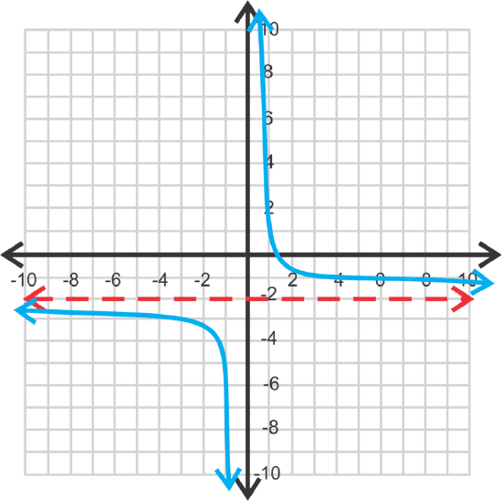
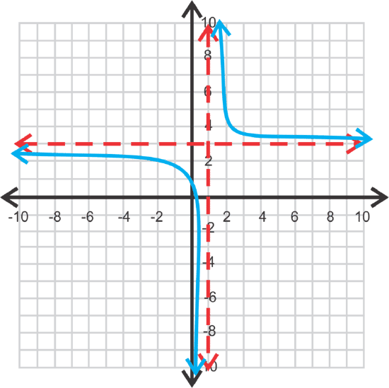
For Examples 3 & 4, graph the rational functions. Find the zero, y-intercept, asymptotes, domain and range.
\(\ y=\frac{4}{x}-2\)
Solution
There is no y-intercept because the y-axis is an asymptote. The other asymptote is y=−2. The domain is all real numbers; x≠0. The range is all real numbers; y≠−2. The zero is:
\(\ \begin{aligned}
0 &=\frac{4}{x}-2 \\
2 &=\frac{4}{x} \\
2 x &=4 \\
x &=2
\end{aligned}\)
\(\ y=\frac{2}{x-1}+3\)
Solution
The asymptotes are x=1 and y=3. Therefore, the domain is all real numbers except 1 and the range is all real numbers except 3. The y-intercept is \(\ y=\frac{2}{0-1}+3=-2+3=1\) and the zero is:
\(\ \begin{aligned}
0 &=\frac{2}{x-1}+3 \\
-3 &=\frac{2}{x-1} \\
-3 x+3 &=2 \\
-3 x &=-1 \rightarrow x=\frac{1}{3}
\end{aligned}\)
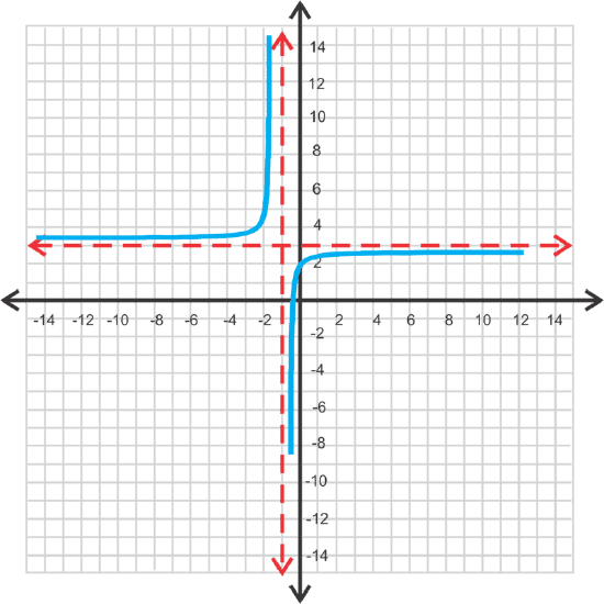
Determine the equation of the hyperbola.
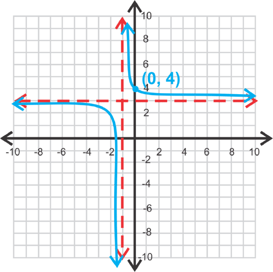
Solution
The asymptotes are x=−1,y=3, making the equation \(\ y=\frac{a}{x+1}+3\). Taking the y-intercept, we can solve for a.
\(\ \begin{aligned}
&4=\frac{a}{0+1}+3 \quad \text { The equation is } y=\frac{1}{x+1}+3\\
&1=a
\end{aligned}\)
Review
- What are the asymptotes for \(\ y=\frac{2}{x+8}-3\)?
- Is (−6,−2) a point on the graph from #1?
- What are the asymptotes for \(\ y=6-\frac{1}{x-4}\)?
- Is (5,4) a point on the graph from #3?
For problems 5-13, graph each rational function, state the equations of the asymptotes, the domain and range and the intercepts.
- \(\ y=\frac{3}{x}\)
- \(\ y=\frac{1}{x}+6\)
- \(\ y=-\frac{1}{x}\)
- \(\ y=-\frac{1}{x+3}\)
- \(\ y=\frac{1}{x+5}\)
- \(\ y=\frac{1}{x-3}-4\)
- \(\ y=\frac{2}{x+4}-3\)
- \(\ y=\frac{5}{x}+2\)
- \(\ y=3-\frac{1}{x+2}\)
Write the equations of the hyperbolas. You may assume that a = 1.
-
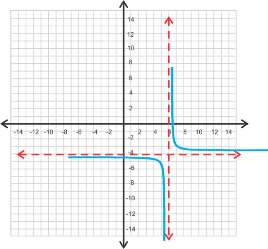 [Figure5]
 -
 [Figure6]
Vocabulary
| Term | Definition |
|---|---|
| Branches | The two curves of a hyperbola are sometimes called branches. |
| hyperbola | A hyperbola is a conic section formed when the cutting plane intersects both sides of the cone, resulting in two infinite “U”-shaped curves. |
| Rational Function | A rational function is any function that can be written as the ratio of two polynomial functions. |
Image Attributions
- [Figure 1]
Credit: NASA's Glenn Research Center
Source: https://en.Wikipedia.org/wiki/File:Boyles_Law_animated.gif;https://www.flickr.com/photos/oddwick/941004365/in/photolist-2r9TPc-cBdwKd-aLq9ek-4ZY5qP-4RPGUc-4ZY3dc-5hDv2p-8faGWS-a4vjvY-513fNw-bqmxDX-bWmB5H-513fGG-bWmB2i-zgcjVy-cdHW8L-89peS3-513fUN-bWmBmD-7Juwon-4wPEDg-bWmAAD-FDyUp-bWmAn4-89peXW-4ZY4YT-bWmAwt-7ED3V-6oDf1e-a73VQD-4ZY32V-62XeHW-cdHX63-9agWUA-8WCXQf-bWmArv-97tmxz-89peLh-G7mc9-bWmATZ-6zuyfQ-89kZnn-bWmBeZ-4F3zbR-tMiQgG-a4stmF-dojsMU-5EQfEd-6S2puk-bzvP78 - [Figure 2]
Credit: NASA's Glenn Research Center
Source: https://en.Wikipedia.org/wiki/File:Boyles_Law_animated.gif;https://www.flickr.com/photos/oddwick/941004365/in/photolist-2r9TPc-cBdwKd-aLq9ek-4ZY5qP-4RPGUc-4ZY3dc-5hDv2p-8faGWS-a4vjvY-513fNw-bqmxDX-bWmB5H-513fGG-bWmB2i-zgcjVy-cdHW8L-89peS3-513fUN-bWmBmD-7Juwon-4wPEDg-bWmAAD-FDyUp-bWmAn4-89peXW-4ZY4YT-bWmAwt-7ED3V-6oDf1e-a73VQD-4ZY32V-62XeHW-cdHX63-9agWUA-8WCXQf-bWmArv-97tmxz-89peLh-G7mc9-bWmATZ-6zuyfQ-89kZnn-bWmBeZ-4F3zbR-tMiQgG-a4stmF-dojsMU-5EQfEd-6S2puk-bzvP78 - [Figure 3]
Credit: NASA's Glenn Research Center
Source: https://en.Wikipedia.org/wiki/File:Boyles_Law_animated.gif;https://www.flickr.com/photos/oddwick/941004365/in/photolist-2r9TPc-cBdwKd-aLq9ek-4ZY5qP-4RPGUc-4ZY3dc-5hDv2p-8faGWS-a4vjvY-513fNw-bqmxDX-bWmB5H-513fGG-bWmB2i-zgcjVy-cdHW8L-89peS3-513fUN-bWmBmD-7Juwon-4wPEDg-bWmAAD-FDyUp-bWmAn4-89peXW-4ZY4YT-bWmAwt-7ED3V-6oDf1e-a73VQD-4ZY32V-62XeHW-cdHX63-9agWUA-8WCXQf-bWmArv-97tmxz-89peLh-G7mc9-bWmATZ-6zuyfQ-89kZnn-bWmBeZ-4F3zbR-tMiQgG-a4stmF-dojsMU-5EQfEd-6S2puk-bzvP78 - [Figure 4]
Credit: NASA's Glenn Research Center
Source: https://en.Wikipedia.org/wiki/File:Boyles_Law_animated.gif;https://www.flickr.com/photos/oddwick/941004365/in/photolist-2r9TPc-cBdwKd-aLq9ek-4ZY5qP-4RPGUc-4ZY3dc-5hDv2p-8faGWS-a4vjvY-513fNw-bqmxDX-bWmB5H-513fGG-bWmB2i-zgcjVy-cdHW8L-89peS3-513fUN-bWmBmD-7Juwon-4wPEDg-bWmAAD-FDyUp-bWmAn4-89peXW-4ZY4YT-bWmAwt-7ED3V-6oDf1e-a73VQD-4ZY32V-62XeHW-cdHX63-9agWUA-8WCXQf-bWmArv-97tmxz-89peLh-G7mc9-bWmATZ-6zuyfQ-89kZnn-bWmBeZ-4F3zbR-tMiQgG-a4stmF-dojsMU-5EQfEd-6S2puk-bzvP78 - [Figure 5]
Credit: NASA's Glenn Research Center
Source: https://en.Wikipedia.org/wiki/File:Boyles_Law_animated.gif;https://www.flickr.com/photos/oddwick/941004365/in/photolist-2r9TPc-cBdwKd-aLq9ek-4ZY5qP-4RPGUc-4ZY3dc-5hDv2p-8faGWS-a4vjvY-513fNw-bqmxDX-bWmB5H-513fGG-bWmB2i-zgcjVy-cdHW8L-89peS3-513fUN-bWmBmD-7Juwon-4wPEDg-bWmAAD-FDyUp-bWmAn4-89peXW-4ZY4YT-bWmAwt-7ED3V-6oDf1e-a73VQD-4ZY32V-62XeHW-cdHX63-9agWUA-8WCXQf-bWmArv-97tmxz-89peLh-G7mc9-bWmATZ-6zuyfQ-89kZnn-bWmBeZ-4F3zbR-tMiQgG-a4stmF-dojsMU-5EQfEd-6S2puk-bzvP78 - [Figure 6]
Source: https://www.flickr.com/photos/oddwick/941004365/in/photolist-2r9TPc-cBdwKd-aLq9ek-4ZY5qP-4RPGUc-4ZY3dc-5hDv2p-8faGWS-a4vjvY-513fNw-bqmxDX-bWmB5H-513fGG-bWmB2i-zgcjVy-cdHW8L-89peS3-513fUN-bWmBmD-7Juwon-4wPEDg-bWmAAD-FDyUp-bWmAn4-89peXW-4ZY4YT-bWmAwt-7ED3V-6oDf1e-a73VQD-4ZY32V-62XeHW-cdHX63-9agWUA-8WCXQf-bWmArv-97tmxz-89peLh-G7mc9-bWmATZ-6zuyfQ-89kZnn-bWmBeZ-4F3zbR-tMiQgG-a4stmF-dojsMU-5EQfEd-6S2puk-bzvP78

