8.5.1: Fundamental Theorem of Calculus

Fundamental Theorem of Calculus

Velocity due to gravity can be easily calculated by the formula: v = gt, where g is the acceleration due to gravity (9.8m/s²) and t is time in seconds. In fact, a decent approximation can be calculated in your head easily by rounding 9.8 to 10 so you can just add a decimal place to the time.

Using this function for velocity, how could you find a function that represented the position of the object after a given time? What about a function that represented the instantaneous acceleration of the object at a given time?

---

Fundamental Theorem of Calculus

Antiderivatives

If you think that evaluating areas under curves is a tedious process you are probably right. Fortunately, there is an easier method. In this section, we shall give a general method of evaluating definite integrals (area under the curve) by using antiderivatives.

Definition: The Antiderivative If F '(x) = f (x), then F '(x) is said to be the antiderivative of f(x).

There are rules for finding the antiderivatives of simple power functions such as f(x) = x². As you read through them, try to think about why they make sense, keeping in mind that differentiation reverses integration.

There are rules for finding the antiderivatives of simple power functions such as f(x) = x². As you read through them, try to think about why they make sense, keeping in mind that differentiation reverses integration.

Rules of Finding the Antiderivatives of Power Functions The Power Rule where C is constant of integration and n is a rational number not equal to -1. A Constant Multiple of a Function Rule where k is a constant. Sum and Difference Rule The Constant Rule
where k is a constant. (Notice that this rule comes as a result of the power rule above.)

The Fundamental Theorem of Calculus

The Fundamental Theorem of Calculus makes the relationship between derivatives and integrals clear. Integration performed on a function can be reversed by differentiation.

The Fundamental Theorem of Calculus If a function f(x) is defined over the interval [a, b] and if F(x) is the antidervative of f on [a, b], then \(\ \begin{aligned} \int_{a}^{b} f(x) d x=\left.F(x)\right|_{a} ^{b} & \\ &=F(b)-F(a) \end{aligned}\)

We can use the relationship between differentiation and integration outlined in the Fundamental Theorem of Calculus to compute definite integrals more quickly.

---

Examples

Example 1

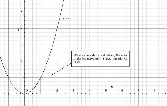
Evaluate \(\ \int_{1}^{2} x^{2} d x\).

Solution

This integral tells us to evaluate the area under the curve \(\ f(x)=x^{2}\), which is a parabola over the interval [1, 2], as shown in the figure below.

To compute the integral according to the Fundamental Theorem of Calculus, we need to find the antiderivative of \(\ f(x)=x^{2}\). It turns out to be \(\ F(x)=(1 / 3) x^{3}+C\), where C is a constant of integration.

How can we get this? Think about the functions that will have derivatives of \(\ x^{2}\). Take the derivative of \(\ F(x)\) to check that we have found such a function. (For more specific rules, see the box after this example). Substituting into the Fundamental Theorem,

\(\ \int_{a}^{b} f(x) d x\)	\(\ =\left.F(x)\right|_{a} ^{b}\)
\(\ \int_{1}^{2} x^{2} d x\)	\(\ =\left[\frac{1}{3} x^{3}+C\right]_{1}^{2}\)
	\(\ =\left[\frac{1}{3}(2)^{3}+C\right]-\left[\frac{1}{3}(1)^{3}+C\right]\)
	\(\ =\left[\frac{8}{3}+C\right]-\left[\frac{1}{3}+C\right]\)
	\(\ =\frac{7}{3}+C-C\)
	\(\ =\frac{7}{3}\)

So the area under the curve is (7/3) units².

Example 2

Evaluate \(\ \int x^{3} d x\)

Solution

Since \(\ \int x^{n} d x=\frac{1}{n+1} x^{n+1}+C\), we have

\(\ \int x^{3} d x\)	\(\ =\frac{1}{3+1} x^{3+1}+C\)
	\(\ =\frac{1}{4} x^{4}+C\)

To check our answer we can take the derivative of \(\ \frac{1}{4} x^{4}+C\) and verify that it is \(\ x^{3}\), the original function in our integral.

Example 3

Evaluate \(\ \int 5 x^{2} d x\)

Solution

Using the constant multiple of a power rule, the coefficient 5 can be removed outside the integral:

\(\ \int 5 x^{2} d x=5 \int x^{2} d x\)

Then we can integrate:

\(\ =5 \cdot \frac{1}{2+1} x^{2+1}+C\)
\(\ =\frac{5}{3} x^{3}+C\)

Again, if we wanted to check our work we could take the derivative of \(\ \frac{5}{3} x^{3}+C\) and verify that we get \(\ 5 x^{2}\).

Example 4

Evaluate \(\ \int\left(3 x^{3}-4 x^{2}+2\right) d x\).

Solution

Using the sum and difference rule we can separate our integral into three integrals:

\(\ \begin{array}{l}
\int\left(3 x^{3}-4 x^{2}+2\right) d x= \\
3\left(\int x^{3} d x\right)-4\left(\int x^{2} d x\right)+\left(\int 2 d x\right) \\
\rightarrow 3 \cdot \frac{1}{4} x^{4}-4 \cdot \frac{1}{3} x^{3}+2 x+C \rightarrow \frac{3}{4} x^{4}-\frac{4}{3} x^{3}+2 x+C
\end{array}\)

Example 5

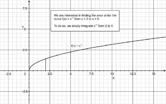
Evaluate \(\ \int_{2}^{5} \sqrt{x} d x\).

Solution

The evaluation of this integral represents calculating the area under the curve \(\ y=\sqrt{x}\) from \(\ x = -2\) to \(\ x = 3\), shown in the figure below.

\(\ \int_{2}^{5} \sqrt{x} d x\)	\(\ =\int_{2}^{5} x^{1 / 2} d x\)
	\(\ =\left[\frac{1}{\frac{1}{2}+1} x^{1 / 2+1}\right]_{2}^{5}\)
	\(\ =\left[\frac{1}{3 / 2} x^{3 / 2}\right]_{2}^{5}\)
	\(\ =\frac{2}{3}\left[x^{3 / 2}\right]_{2}^{5}\)
	\(\ =\frac{2}{3}\left[5^{3 / 2}-2^{3 / 2}\right]\)
	\(\ =5.57\)

So the area under the curve is 5.57.

Example 6

Use the Fundamental Theorem of Calculus to solve: \(\ \int_{4}^{6} \frac{d x}{x}\).

Solution

Given what we know, that if \(\ F(x)=\ln x\), then \(\ F^{\prime}(x)=\frac{1}{x}\)

Thus, we apply the Fundamental Theorem of Calculus:

\(\ \int-4^{6} \frac{d x}{x}=\ln x \mid-46\)

= F(6) - F(4) = [ln(6)] - [ln(4)] = 0.4055

Example 7

Use the Fundamental Theorem of Calculus to solve: \(\ \int_{-2 p}^{2 p} 3 \cos (x) d x\).

Solution

Given what we know, that if F(x) = 3sin(x), then F'(x) = 3cos(x)

So we apply the Fundamental Theorem of Calculus:

\(\ \int_{-2 p}^{2 p} 3 \cos d x=\left.3 \sin (x)\right|_{-2 p} ^{2 p}\)

= F(8) - F(0) = [3sin(2p)] - [3sin(-2p)] = 1 - 0 = 0

---

Review

Evaluate the integral:

1. Evaluate the integral \(\ \int_{0}^{3} 5 x d x\)
2. Evaluate the integral \(\ \int_{0}^{1} x^{4} d x\)
3. Evaluate the integral \(\ \int_{1}^{4}(x-3) d x\)

Find the integral:

4. Find the integral of (x + 1)(2x - 3) from -1 to 2.
5. Find the integral of \(\ \sqrt{x}\) from 0 to 9.
6. Find \(\ \int_{-1}^{0}-3 d x\)
7. Find \(\ \int_{-1}^{3} d x\)
8. Find \(\ \int_{-p}^{\frac{p}{2}}-4 \cos (x) d x\)
9. Find \(\ \int_{0}^{2}-d x\)
10. Find \(\ \int_{2}^{7} \frac{d x}{x}\)
11. Find \(\ \int_{-2}^{0} x+5 d x\)
12. Find \(\ \int_{-p}^{\frac{3 p}{2}} 6 \sin (x) d x\)
13. Find \(\ \int_{6}^{7} \frac{d x}{x}\)

Challenge yourself:

14. Sketch \(\ y=x^{3}\) and \(\ y=x\) on the same coordinate system and then find the area of the region enclosed between them (a) in the first quadrant and (b) in the first and third quadrants.
15. Evaluate the integral \(\ \int_{-R}^{R}\left(\pi R^{2}-\pi x^{2}\right) d x\) where R is a constant.

---

Review (Answers)

To see the Review answers, open this PDF file and look for section 8.13.

---

Vocabulary

Term	Definition
antiderivative	An antiderivative is a function that reverses a derivative. Function A is the antiderivative of function B if function B is the derivative of function A.
derivative	The derivative of a function is the slope of the line tangent to the function at a given point on the graph. Notations for derivative include \(\ f^{\prime}(x), \frac{d y}{d x}, y^{\prime}, \frac{d f}{d x}\) and \(\ \frac{df(x)}{dx}\).
fundamental theorem of calculus	The fundamental theorem of calculus demonstrates that integration performed on a function can be reversed by differentiation.
integral	An integral is used to calculate the area under a curve or the area between two curves.
theorem	A theorem is a statement that can be proven true using postulates, definitions, and other theorems that have already been proven.