4.3: Tangent Line Approximation
- Page ID
- 1246
\( \newcommand{\vecs}[1]{\overset { \scriptstyle \rightharpoonup} {\mathbf{#1}} } \)
\( \newcommand{\vecd}[1]{\overset{-\!-\!\rightharpoonup}{\vphantom{a}\smash {#1}}} \)
\( \newcommand{\dsum}{\displaystyle\sum\limits} \)
\( \newcommand{\dint}{\displaystyle\int\limits} \)
\( \newcommand{\dlim}{\displaystyle\lim\limits} \)
\( \newcommand{\id}{\mathrm{id}}\) \( \newcommand{\Span}{\mathrm{span}}\)
( \newcommand{\kernel}{\mathrm{null}\,}\) \( \newcommand{\range}{\mathrm{range}\,}\)
\( \newcommand{\RealPart}{\mathrm{Re}}\) \( \newcommand{\ImaginaryPart}{\mathrm{Im}}\)
\( \newcommand{\Argument}{\mathrm{Arg}}\) \( \newcommand{\norm}[1]{\| #1 \|}\)
\( \newcommand{\inner}[2]{\langle #1, #2 \rangle}\)
\( \newcommand{\Span}{\mathrm{span}}\)
\( \newcommand{\id}{\mathrm{id}}\)
\( \newcommand{\Span}{\mathrm{span}}\)
\( \newcommand{\kernel}{\mathrm{null}\,}\)
\( \newcommand{\range}{\mathrm{range}\,}\)
\( \newcommand{\RealPart}{\mathrm{Re}}\)
\( \newcommand{\ImaginaryPart}{\mathrm{Im}}\)
\( \newcommand{\Argument}{\mathrm{Arg}}\)
\( \newcommand{\norm}[1]{\| #1 \|}\)
\( \newcommand{\inner}[2]{\langle #1, #2 \rangle}\)
\( \newcommand{\Span}{\mathrm{span}}\) \( \newcommand{\AA}{\unicode[.8,0]{x212B}}\)
\( \newcommand{\vectorA}[1]{\vec{#1}} % arrow\)
\( \newcommand{\vectorAt}[1]{\vec{\text{#1}}} % arrow\)
\( \newcommand{\vectorB}[1]{\overset { \scriptstyle \rightharpoonup} {\mathbf{#1}} } \)
\( \newcommand{\vectorC}[1]{\textbf{#1}} \)
\( \newcommand{\vectorD}[1]{\overrightarrow{#1}} \)
\( \newcommand{\vectorDt}[1]{\overrightarrow{\text{#1}}} \)
\( \newcommand{\vectE}[1]{\overset{-\!-\!\rightharpoonup}{\vphantom{a}\smash{\mathbf {#1}}}} \)
\( \newcommand{\vecs}[1]{\overset { \scriptstyle \rightharpoonup} {\mathbf{#1}} } \)
\(\newcommand{\longvect}{\overrightarrow}\)
\( \newcommand{\vecd}[1]{\overset{-\!-\!\rightharpoonup}{\vphantom{a}\smash {#1}}} \)
\(\newcommand{\avec}{\mathbf a}\) \(\newcommand{\bvec}{\mathbf b}\) \(\newcommand{\cvec}{\mathbf c}\) \(\newcommand{\dvec}{\mathbf d}\) \(\newcommand{\dtil}{\widetilde{\mathbf d}}\) \(\newcommand{\evec}{\mathbf e}\) \(\newcommand{\fvec}{\mathbf f}\) \(\newcommand{\nvec}{\mathbf n}\) \(\newcommand{\pvec}{\mathbf p}\) \(\newcommand{\qvec}{\mathbf q}\) \(\newcommand{\svec}{\mathbf s}\) \(\newcommand{\tvec}{\mathbf t}\) \(\newcommand{\uvec}{\mathbf u}\) \(\newcommand{\vvec}{\mathbf v}\) \(\newcommand{\wvec}{\mathbf w}\) \(\newcommand{\xvec}{\mathbf x}\) \(\newcommand{\yvec}{\mathbf y}\) \(\newcommand{\zvec}{\mathbf z}\) \(\newcommand{\rvec}{\mathbf r}\) \(\newcommand{\mvec}{\mathbf m}\) \(\newcommand{\zerovec}{\mathbf 0}\) \(\newcommand{\onevec}{\mathbf 1}\) \(\newcommand{\real}{\mathbb R}\) \(\newcommand{\twovec}[2]{\left[\begin{array}{r}#1 \\ #2 \end{array}\right]}\) \(\newcommand{\ctwovec}[2]{\left[\begin{array}{c}#1 \\ #2 \end{array}\right]}\) \(\newcommand{\threevec}[3]{\left[\begin{array}{r}#1 \\ #2 \\ #3 \end{array}\right]}\) \(\newcommand{\cthreevec}[3]{\left[\begin{array}{c}#1 \\ #2 \\ #3 \end{array}\right]}\) \(\newcommand{\fourvec}[4]{\left[\begin{array}{r}#1 \\ #2 \\ #3 \\ #4 \end{array}\right]}\) \(\newcommand{\cfourvec}[4]{\left[\begin{array}{c}#1 \\ #2 \\ #3 \\ #4 \end{array}\right]}\) \(\newcommand{\fivevec}[5]{\left[\begin{array}{r}#1 \\ #2 \\ #3 \\ #4 \\ #5 \\ \end{array}\right]}\) \(\newcommand{\cfivevec}[5]{\left[\begin{array}{c}#1 \\ #2 \\ #3 \\ #4 \\ #5 \\ \end{array}\right]}\) \(\newcommand{\mattwo}[4]{\left[\begin{array}{rr}#1 \amp #2 \\ #3 \amp #4 \\ \end{array}\right]}\) \(\newcommand{\laspan}[1]{\text{Span}\{#1\}}\) \(\newcommand{\bcal}{\cal B}\) \(\newcommand{\ccal}{\cal C}\) \(\newcommand{\scal}{\cal S}\) \(\newcommand{\wcal}{\cal W}\) \(\newcommand{\ecal}{\cal E}\) \(\newcommand{\coords}[2]{\left\{#1\right\}_{#2}}\) \(\newcommand{\gray}[1]{\color{gray}{#1}}\) \(\newcommand{\lgray}[1]{\color{lightgray}{#1}}\) \(\newcommand{\rank}{\operatorname{rank}}\) \(\newcommand{\row}{\text{Row}}\) \(\newcommand{\col}{\text{Col}}\) \(\renewcommand{\row}{\text{Row}}\) \(\newcommand{\nul}{\text{Nul}}\) \(\newcommand{\var}{\text{Var}}\) \(\newcommand{\corr}{\text{corr}}\) \(\newcommand{\len}[1]{\left|#1\right|}\) \(\newcommand{\bbar}{\overline{\bvec}}\) \(\newcommand{\bhat}{\widehat{\bvec}}\) \(\newcommand{\bperp}{\bvec^\perp}\) \(\newcommand{\xhat}{\widehat{\xvec}}\) \(\newcommand{\vhat}{\widehat{\vvec}}\) \(\newcommand{\uhat}{\widehat{\uvec}}\) \(\newcommand{\what}{\widehat{\wvec}}\) \(\newcommand{\Sighat}{\widehat{\Sigma}}\) \(\newcommand{\lt}{<}\) \(\newcommand{\gt}{>}\) \(\newcommand{\amp}{&}\) \(\definecolor{fillinmathshade}{gray}{0.9}\)Suppose you absolutely needed to know the value of the square root of 19 but all you had was pencil and paper, no calculator. Could you calculate it? With your current understanding of the derivative as the slope of a tangent line, you should be able to. Try computing 190.5 without a calculator; then compare your result with this concepts method of linearization and a calculator.
Linearization
Linearization of a function means using the tangent line of a function at a point as an approximation to the function in the vicinity of the point. This relationship between a tangent and a graph at the point of tangency is often referred to as local linearization.
Given the function f(x) and the derivative f′(x), the tangent line at a point x0 can be written in point-slope form as:
y−f(x0)=f′(x0)(x−x0) or y=f(x0)+f′(x0)(x−x0).
If we consider that this tangent line is a good approximation to f(x) in the vicinity of x0, we can write
f(x)≈y=f(x0)+f′(x0)(x−x0). This is the linearization of f(x) about x0.
The tangent line as the local linearization of f(x) is often designated L(x), so that
f(x)≈L(x)=f(x0)+f′(x0)(x−x0).
Take the function f(x)=x2−2x−3 and find the linearization at the points x0=1.5 and x0=−0.5.
The linearization of f(x) is given by: f(x)≈f(x0)+f′(x0)(x−x0).
We have:
f(1.5)=−3.75 and f(−0.5)=−1.75
f′(x)=2x−2, so that f′(1.5)=1 and f′(−0.5)=−3.
The linearization becomes:

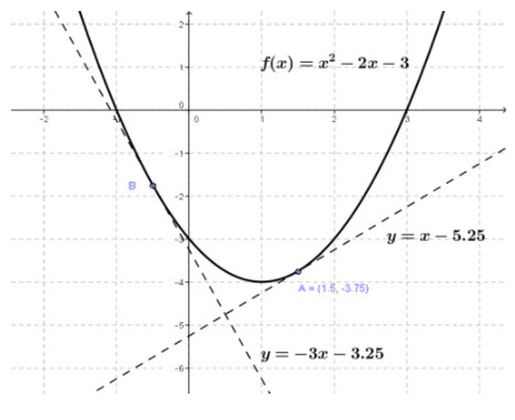
As the figure illustrates and the table shows, as we move away from x0, we lose accuracy.
| Error near x0=−0.5 | Error near x0=1.5 | ||||||
| x | f(x) | −3x−3.25 | |True-Approx| | x | f(x) | x−5.25 | |True-Approx| |
| -1 | 0 | -0.25 | 0.25 | 1.0 | -4 | -4.25 | 0.25 |
| -0.5 | -1.75 | -1.75 | 0.00 | 1.5 | -3.75 | -3.75 | 0.00 |
| 0 | -3 | -3.25 | 0.25 | 2.0 | -3.25 | -3.00 | 0.25 |
Examples
Example 1
Earlier, you were asked to first try computing 190.5 without a calculator and then to compare your result with this concepts method of linearization and a calculator.
Congratulations if you were able to linearize x0.5 at x=16( or x=25).
The linearization is y=1/8(x−16)+4, which means y=4.375 when x=19. A calculator would give 4.359.
Example 2
Find the linearization of f(x)=(x+3)0.5 at point x=−1.
The linearization of f(x) is given by: f(x)≈f(x0)+f′(x0)(x−x0).
We have:
f(1)=2, and
f′(x)=1/2(x+3)−1/2, so that f′(1)=1/4.
The linearization becomes:
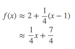
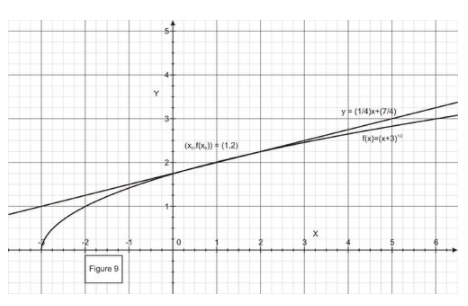
This tells us that near the point x=1, the function f(x)=(x+3)0.5 approximates the line y=(x/4)+7/4. As the figure illustrates and the table shows, as we move away from x=1, we lose accuracy.
CC BY-NC-SA
| x | f(x) | ≈14x+74 |
|True-Approx| |
|
1 |
2 |
2 |
0 |
|
1.5 |
2.121 |
2.125 |
0.004 |
|
2 |
2.236 |
2.25 |
0.014 |
|
3 |
2.449 |
2.5 |
0.41 |
Example 3
Find the linearization of y=sinx at x=π/3.
The linearization of f(x) is given by: f(x)≈f(x0)+f′(x0)(x−x0).
We have

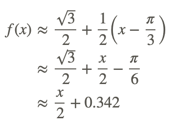
The linearization becomes:
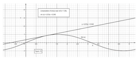
CC BY-NC-SA
Example 4
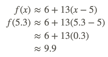
Let f be a function such that f(5)=6 and whose derivative is f′(x)=(x3+44)0.5. Approximate f(5.3).
The linearization of f(x) is given by: f(x)≈f(x0)+f′(x0)(x−x0).
Since we have f(5)=6, let x0=5.
Then f′(x0)=(x03+44)0.5=1690.5=13
The linearization becomes:
Review
- Find the linearization of f(x)=x2+1/x, x0=1, f(1.7)
- Find the linearization of f(x)=tanx at a=π.
- Use the linearization method to show that when x≪1 (much less than1), then (1+x)n≈1+nx.
- Use the result of problem #3, (1+x)n≈1+nx, to find the approximation for the following:
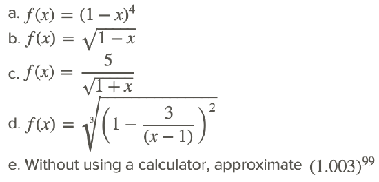
For #5 - 13, find the linearization of the given function at the given point x0 and use this approximation to compute the given quantity. Compare the result to the value obtained by calculator; compute the error.
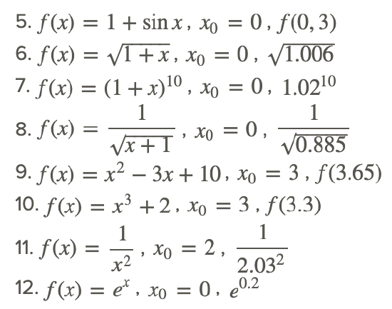
For #13 - 14, estimate the following numbers and determine the error:

Vocabulary
| Term | Definition |
|---|---|
| linearization | Local linearization of a function means to approximate the function at a point by the tangent line at the point. |
Additional Resources
PLIX: Play, Learn, Interact, eXplore - Estimating square roots
Video: Calculus - Linear Approximation
Practice: Tangent Line Approximation
Real World: On Autopilot

