
9.3: Area Sums
- Page ID
- 1258
\( \newcommand{\vecs}[1]{\overset { \scriptstyle \rightharpoonup} {\mathbf{#1}} } \)
\( \newcommand{\vecd}[1]{\overset{-\!-\!\rightharpoonup}{\vphantom{a}\smash {#1}}} \)
\( \newcommand{\dsum}{\displaystyle\sum\limits} \)
\( \newcommand{\dint}{\displaystyle\int\limits} \)
\( \newcommand{\dlim}{\displaystyle\lim\limits} \)
\( \newcommand{\id}{\mathrm{id}}\) \( \newcommand{\Span}{\mathrm{span}}\)
( \newcommand{\kernel}{\mathrm{null}\,}\) \( \newcommand{\range}{\mathrm{range}\,}\)
\( \newcommand{\RealPart}{\mathrm{Re}}\) \( \newcommand{\ImaginaryPart}{\mathrm{Im}}\)
\( \newcommand{\Argument}{\mathrm{Arg}}\) \( \newcommand{\norm}[1]{\| #1 \|}\)
\( \newcommand{\inner}[2]{\langle #1, #2 \rangle}\)
\( \newcommand{\Span}{\mathrm{span}}\)
\( \newcommand{\id}{\mathrm{id}}\)
\( \newcommand{\Span}{\mathrm{span}}\)
\( \newcommand{\kernel}{\mathrm{null}\,}\)
\( \newcommand{\range}{\mathrm{range}\,}\)
\( \newcommand{\RealPart}{\mathrm{Re}}\)
\( \newcommand{\ImaginaryPart}{\mathrm{Im}}\)
\( \newcommand{\Argument}{\mathrm{Arg}}\)
\( \newcommand{\norm}[1]{\| #1 \|}\)
\( \newcommand{\inner}[2]{\langle #1, #2 \rangle}\)
\( \newcommand{\Span}{\mathrm{span}}\) \( \newcommand{\AA}{\unicode[.8,0]{x212B}}\)
\( \newcommand{\vectorA}[1]{\vec{#1}} % arrow\)
\( \newcommand{\vectorAt}[1]{\vec{\text{#1}}} % arrow\)
\( \newcommand{\vectorB}[1]{\overset { \scriptstyle \rightharpoonup} {\mathbf{#1}} } \)
\( \newcommand{\vectorC}[1]{\textbf{#1}} \)
\( \newcommand{\vectorD}[1]{\overrightarrow{#1}} \)
\( \newcommand{\vectorDt}[1]{\overrightarrow{\text{#1}}} \)
\( \newcommand{\vectE}[1]{\overset{-\!-\!\rightharpoonup}{\vphantom{a}\smash{\mathbf {#1}}}} \)
\( \newcommand{\vecs}[1]{\overset { \scriptstyle \rightharpoonup} {\mathbf{#1}} } \)
\(\newcommand{\longvect}{\overrightarrow}\)
\( \newcommand{\vecd}[1]{\overset{-\!-\!\rightharpoonup}{\vphantom{a}\smash {#1}}} \)
\(\newcommand{\avec}{\mathbf a}\) \(\newcommand{\bvec}{\mathbf b}\) \(\newcommand{\cvec}{\mathbf c}\) \(\newcommand{\dvec}{\mathbf d}\) \(\newcommand{\dtil}{\widetilde{\mathbf d}}\) \(\newcommand{\evec}{\mathbf e}\) \(\newcommand{\fvec}{\mathbf f}\) \(\newcommand{\nvec}{\mathbf n}\) \(\newcommand{\pvec}{\mathbf p}\) \(\newcommand{\qvec}{\mathbf q}\) \(\newcommand{\svec}{\mathbf s}\) \(\newcommand{\tvec}{\mathbf t}\) \(\newcommand{\uvec}{\mathbf u}\) \(\newcommand{\vvec}{\mathbf v}\) \(\newcommand{\wvec}{\mathbf w}\) \(\newcommand{\xvec}{\mathbf x}\) \(\newcommand{\yvec}{\mathbf y}\) \(\newcommand{\zvec}{\mathbf z}\) \(\newcommand{\rvec}{\mathbf r}\) \(\newcommand{\mvec}{\mathbf m}\) \(\newcommand{\zerovec}{\mathbf 0}\) \(\newcommand{\onevec}{\mathbf 1}\) \(\newcommand{\real}{\mathbb R}\) \(\newcommand{\twovec}[2]{\left[\begin{array}{r}#1 \\ #2 \end{array}\right]}\) \(\newcommand{\ctwovec}[2]{\left[\begin{array}{c}#1 \\ #2 \end{array}\right]}\) \(\newcommand{\threevec}[3]{\left[\begin{array}{r}#1 \\ #2 \\ #3 \end{array}\right]}\) \(\newcommand{\cthreevec}[3]{\left[\begin{array}{c}#1 \\ #2 \\ #3 \end{array}\right]}\) \(\newcommand{\fourvec}[4]{\left[\begin{array}{r}#1 \\ #2 \\ #3 \\ #4 \end{array}\right]}\) \(\newcommand{\cfourvec}[4]{\left[\begin{array}{c}#1 \\ #2 \\ #3 \\ #4 \end{array}\right]}\) \(\newcommand{\fivevec}[5]{\left[\begin{array}{r}#1 \\ #2 \\ #3 \\ #4 \\ #5 \\ \end{array}\right]}\) \(\newcommand{\cfivevec}[5]{\left[\begin{array}{c}#1 \\ #2 \\ #3 \\ #4 \\ #5 \\ \end{array}\right]}\) \(\newcommand{\mattwo}[4]{\left[\begin{array}{rr}#1 \amp #2 \\ #3 \amp #4 \\ \end{array}\right]}\) \(\newcommand{\laspan}[1]{\text{Span}\{#1\}}\) \(\newcommand{\bcal}{\cal B}\) \(\newcommand{\ccal}{\cal C}\) \(\newcommand{\scal}{\cal S}\) \(\newcommand{\wcal}{\cal W}\) \(\newcommand{\ecal}{\cal E}\) \(\newcommand{\coords}[2]{\left\{#1\right\}_{#2}}\) \(\newcommand{\gray}[1]{\color{gray}{#1}}\) \(\newcommand{\lgray}[1]{\color{lightgray}{#1}}\) \(\newcommand{\rank}{\operatorname{rank}}\) \(\newcommand{\row}{\text{Row}}\) \(\newcommand{\col}{\text{Col}}\) \(\renewcommand{\row}{\text{Row}}\) \(\newcommand{\nul}{\text{Nul}}\) \(\newcommand{\var}{\text{Var}}\) \(\newcommand{\corr}{\text{corr}}\) \(\newcommand{\len}[1]{\left|#1\right|}\) \(\newcommand{\bbar}{\overline{\bvec}}\) \(\newcommand{\bhat}{\widehat{\bvec}}\) \(\newcommand{\bperp}{\bvec^\perp}\) \(\newcommand{\xhat}{\widehat{\xvec}}\) \(\newcommand{\vhat}{\widehat{\vvec}}\) \(\newcommand{\uhat}{\widehat{\uvec}}\) \(\newcommand{\what}{\widehat{\wvec}}\) \(\newcommand{\Sighat}{\widehat{\Sigma}}\) \(\newcommand{\lt}{<}\) \(\newcommand{\gt}{>}\) \(\newcommand{\amp}{&}\) \(\definecolor{fillinmathshade}{gray}{0.9}\)Finding the area under the curve of a function, f(x), is one of the central problems that arises in Calculus. You already know how to compute the area of some simple function curve shapes using geometric formulas, and can sometimes quickly use these methods. But, what would you do if the function curves were more complex? The key approach of calculus is to take a simple method, apply it on a small scale, and then take it to the limit at infinity.
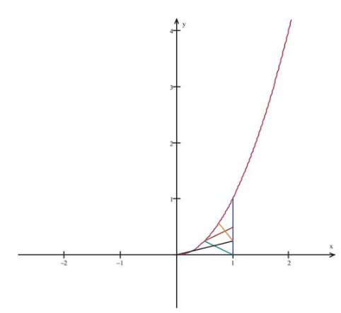
To gain some insight into the idea of finding the area under a curve, do the following before you go further: take a simple parabola curve (concave up and positive), divide an interval on the x-axis into a number of equal subintervals, and draw a rectangle in each subinterval that intersects the parabola. The summation of the rectangles would be an area estimate. How many different types of intersections can a rectangle make with the parabola? Can you say anything about how the intersection under or over estimates the area underneath the curve? Can you see that the more rectangles used for a given interval, the better the estimate?
Riemann Sums
For simple functions like f(x)=c(c>0), or f(x)=cx (c is a constant >0) over some interval [0,x0], we can use simple geometry to get the area under each curve (try confirming this on your own):
- For f(x)=c(c>0); the area A is that of a simple rectangle, A=cx0.
- For f(x)=cx(c>0); the area A is that of a simple triangle, \( A=\frac{1}{2}x_0(cx_0)=c\frac{x_0^2}{2} \nonumber\).
How can the area be determined for more complex functions?
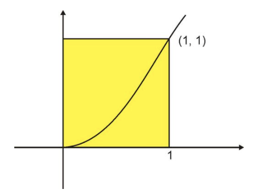
Let’s consider our basic quadratic function \( f(x)=x^2 \nonumber\). Suppose we are interested in finding the area, A, under the curve from x=0 to x=1. The area we are talking about is the cross-hatched space under the curve shown below.
CC BY-NC-SA
One way to estimate the area under the curve is to compute the area of the square that has a corner at (1, 1) as shown below, and then take half.
CC BY-NC-SA
This gives an area \( A=\frac{1}{2} \nonumber\). This is a good first estimate of the area; the exact answer will be shown to be \( A=\frac{1}{3} \nonumber\).
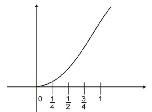
How can we make a better estimate? How about dividing the x-interval from x=0 to x=1 into multiple sub-intervals of equal widths.
Let’s look at problems each having more subintervals than the previous one.
4 equal subintervals:
Start by using four such subintervals as indicated:
We now will construct four rectangles that will serve as the basis for our approximation of the area. The subintervals will serve as the width of the rectangles. We will take the length of each rectangle to be the maximum value of the function in the subinterval. (We could also choose the minimum or midpoint value of the function in the subinterval.)
Hence we get the following figure:
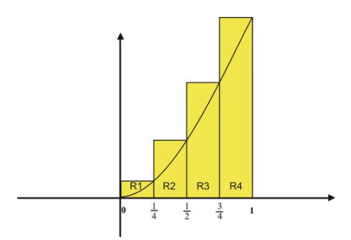
If we call the rectangles R1−R4, from left to right, then we have the areas
Finding the area under the curve of a function, f(x), is one of the central problems that arises in Calculus. You already know how to compute the area of some simple function curve shapes using geometric formulas, and can sometimes quickly use these methods. But, what would you do if the function curves were more complex? The key approach of calculus is to take a simple method, apply it on a small scale, and then take it to the limit at infinity.
To gain some insight into the idea of finding the area under a curve, do the following before you go further: take a simple parabola curve (concave up and positive), divide an interval on the x-axis into a number of equal subintervals, and draw a rectangle in each subinterval that intersects the parabola. The summation of the rectangles would be an area estimate. How many different types of intersections can a rectangle make with the parabola? Can you say anything about how the intersection under or over estimates the area underneath the curve? Can you see that the more rectangles used for a given interval, the better the estimate?
8 Equal Sub-intervals:
f we divide the interval into 8 equal sub-intervals, the width of each rectangle is now w=18.
The area estimate now becomes:
\[ A≈R_1+R_2+R_3+R_4+R_5+R_6+R_7+R_8 \nonumber\]
\[ ≈ \sum_{i=1}^8 R_i \nonumber\] Use of Sigma Notation
\[ ≈\frac{1}{512}+\frac{4}{512}+\frac{9}{512}+\frac{16}{512}+\frac{25}{512}+\frac{36}{512}+\frac{49}{512}+\frac{64}{512} \nonumber\]
\[ ≈\frac{204}{512} \nonumber\]
\[ A≈0.3984 \nonumber\]
Note that the Sigma Notation \( (\sum_{i=1}^8 R_i) \nonumber\) used above enables us to indicate the sum of the individual rectangle areas without the need to write out all of the individual terms. The sigma symbol with these indices tells us how the rectangles are labeled and how many terms are in the sum.
In addition, the summation of rectangles that gives the area approximation could be written in the following general form:
\[ A≈R=\sum_{i=1}^n R_i= \sum_{i=1}^n f(w_i)(x_i−x_{i−1})=\sum_{i=1}^n f(w_i)Δx_i \nonumber\]
where we choose the value of n to be as large as we want, wi to be any value of x in the interval \( (x_i−x_i−1)\nonumber\), and \( (x_i−x_i−1) \nonumber\) to be the i-th of n subintervals (not necessarily equal) in the interval [a,b] that f is defined on. This type of summation is called a Riemann sum.
16 equal sub-intervals:
If we now divide the interval into 16 equal sub-intervals, the width of each rectangle is now \( w=\frac{1}{16} \nonumber\).
The area estimate now becomes:
\[ A≈R_1+R_2+R_3+R_4+R_5+⋯+R_{16} \nonumber\]
\[ ≈\sum_{i=1}^{16} R_i \nonumber\] Use of Sigma Notation
\[ ≈\frac{1}{4096}+\frac{4}{4096}+\frac{9}{4096}+⋯+\frac{196}{4096}+\frac{225}{4096}+\frac{256}{4096} \nonumber\]
\[ ≈\frac{1496}{4096} \nonumber\]
\[ A≈0.3652 \nonumber\]
Again, the sigma notation has been used to eliminate the need to write out all of the individual terms.
The table gives a summary of the area estimate results so far.
|
Sub-intervals |
Area Estimate |
|
1 |
1 (0.5) |
|
4 |
0.4688 |
|
8 |
0.3984 |
|
16 |
0.3652 |
Intuitively, we have the feeling that we can improve the area approximation by sub-dividing the interval from x=0 to x=1 into more and more sub-intervals, thus creating successively smaller and smaller rectangles to refine our estimates.
We are now ready to formalize the use of sums to compute areas.
First, we define lower and upper sums:
Let f be a bounded function in a closed interval [a,b] and \( P=[x_0,…,x_n] \nonumber\) the partition of [a,b] into n subintervals.
Define the lower and upper sums, respectively, over partition P, by
\[ S(P)=\sum_{1}^{n} m_i(x_i−x_{i−1})=m_1(x_1−x_0)+m_2(x_2−x_1)++m_n(x_n−x_{n−1}) \nonumber\]
\[ T(P)= \sum_1^n M_i(x_i−x_{i−1})=M1_(x_1−x_0)+M_2(x_2−x_1)+…+M_n(x_n−x_{n−1}) \nonumber\]
where mi is the minimum value of f in the interval of length \( x_i−x_{i−1} \nonumber\) and \( M_i \nonumber\) is the maximum value of f in the interval of length \( x_i−x_{i−1} \nonumber\).
S(P) and T(P) are Riemann sums, where mi and Mi are particular choices for wi in the general Riemann sum formulation above.
Next, we will link area under a curve with the limit of the lower or upper sums for an increasingly large number of subintervals:
Let f be a continuous non-negative function on a closed interval [a,b]. Let P be a partition of n equal sub intervals over [a,b]. Then the area under the curve of f is the limit of the upper and lower sums, that is
\[ A= \lim_{n \to +∞} S(P)= \lim_{n \to +∞}T(P) \nonumber\]
The following problem shows how we can use these definitions to find the area under a curve.
Show that the limit of upper sum for the function \( f(x)=x^2 \nonumber\), from \( x=0 \mbox{ to } x=x_0 \nonumber\), approaches the value \( A=\frac{x_0^3}{3} \nonumber\).
Let P be a partition of n equal sub intervals over \( [0,x_0] \nonumber\). By definition we have
\[ T(P)= \sum{1}^{n} M_i(x_i−x_{i−1})=M_1(x_1−x_0)+M_2(x_2−x_1)+…+M_n(x_n−x_{n−1}) \nonumber\]
Each rectangle will have width \( \frac{x_0}{n} \nonumber\), so that the evaluation of T(P) is: \( T(P)= \sum_{1}^{n} M_i(x_i−x_{i−1}) \nonumber\)
\( = M_2(x_2−x_1)+…+M_n(x_n−x_{n−1}) \nonumber\)
\( =(\frac{x_0}{n})2\frac{x_0}{n}+(2\frac{x_0}{n})2\frac{x_0}{n}+…+(n\frac{x_0}{n})2\frac{x_0}{n} \nonumber\) Equal length sub-intervals.
\( =(\frac{x_0}{n})^2\frac{x_0}{n}(1^2+2^2+3^2+…+n^2) \nonumber\)
\( =(\frac{x_0}{n})^3(1^2+2^2+3^2+…+n^2) \nonumber\)
\( =(\frac{x_0^3}{n})^3(\frac{n(n+1)(2n+1)}{6}) \nonumber\) Makes use of: \( \sum_{i=1}^{n} i^2=\frac{n(n+1)(2n+1)}{6} \nonumber\)
\( =(\frac{x_0^3}{6})(\frac{n(n+1)(2n+1)}{n^3}) \nonumber\)
\(=(\frac{x_0^3}{6})(1+\frac{1}{n})(2+\frac{1}{n}) \nonumber\)
Observe that:
\[ \lim_{n \to ∞} [(\frac{x_0^3}{6})(1+\frac{1}{n})(2+\frac{1}{n})]=(\frac{x_0^3}{6})⋅2=\frac{x_0^3}{3} \nonumber\]
The area, A, under the curve of the function \( f(x)=x^2 \nonumber\) from \( x=0 \mbox{ to } x=x_0 \nonumber\), approaches the value \( A=\frac{x_0^3}{3} \nonumber\). Note that if x0=1, we get the result A=13. Compare this value to the results from the previous problem.
The same approach to determine the area can be used with S(P), and it yields the same result, \( A = \frac{x_0^3}{3} \nonumber\).
Examples
Example 1
Earlier, you were asked about using rectangles to estimate the area under a curve. How many different types of intersections can a rectangle make with the parabola? Can you say anything about how the intersection under or over estimates the area underneath the curve? Can you see that the more rectangles used (smaller subinterval) for a given interval, the better the area estimate?
Where your rectangle intersects the parabola establishes the height of the rectangle, and just depends on the value of x within the subinterval: left end of rectangle (beginning of sub-interval), right end of rectangle (end of subinterval), or anywhere in between. For this concave up parabola, you should be able to see that using a left-end rectangle underestimates the area under the parabola; a right-end rectangle overestimates the area. A rectangle with height somewhere in between, say at the mid-point, might overestimate a portion and underestimate a portion, i.e., provide a better area estimate.
Example 2
Use the limit definition of area to find the area under the function f(x)=4−x from 1 to x=3.
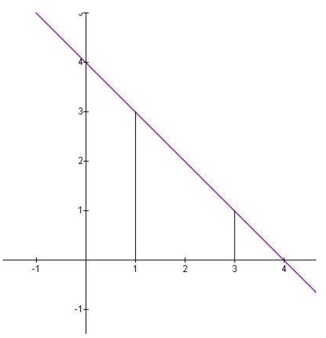
If we partition the interval [1,3] into n equal sub-intervals, then each sub-interval will have length \( \frac{3−1}{n}=\frac{2}{n} \nonumber\), and height 3−i△x as i varies from 1 to n. So we have \( △x=\frac{2}{n} \nonumber\) and
\( S(P)= \sum_1^n m_i(x_i−x_{i−1}) \nonumber\) Lower sum using minimum function value in each subinterval.
\( = \sum_1^n (3−i\frac{2}{n})\frac{2}{n} \nonumber\)
\( S(P)= \sum_1^n m_i(x_i−x_{i−1}) \nonumber\) Sub-intervals of equal length.
\( = \sum_1^n (3⋅\frac{2}{n})− \sum_1^n i(\frac{2}{n})^2 \nonumber\)
\( =6−(\frac{2}{n})^2 \sum_1^n i \nonumber\)
\( =6−(\frac{2}{n})^2⋅(\frac{n(n+1)}{2}) \nonumber\) Makes use of:
\( =6−2⋅(\frac{n(n+1)}{n^2}) \sum_{i=1}^n i=\frac{n(n+1)}{2} \nonumber\)
\( S(P)=6−2⋅(1+\frac{1}{n}) \nonumber\)
Observe that:
\[ \lim_{n \to ∞} [6−2⋅(1+\frac{1}{n})]=6−2=4 \nonumber\]
The area, A, under the curve of the function approaches the value A=4. The same approach can be used with S(P), yielding the same result.
Of course this example may also be solved with simple geometry. It is left to the reader to confirm that the two methods yield the same area.
Review
For #1-3, find S(P) and T(P) under the partition P.
- \( f(x)=1−x^2, P={0,12,1,32,2} \nonumber\)
- \( f(x)=2x^2, P={−1,−12,0,12,1} \nonumber\)
- \( f(x)=\frac{1}{x}, P={−4,−3,−2,−1} \nonumber\)
- Consider f(x)=2−x from x=0 to x=2. Use Riemann Sums with four subintervals of equal lengths. Choose the midpoints of each subinterval as the sample points.
- Repeat problem #1 using geometry to calculate the exact area of the region under the graph of f(x)=2−x from x=0 to x=2. (Hint: Sketch a graph of the region and see if you can compute its area using area measurement formulas from geometry.)
- Repeat problem #4 using the definition of the definite integral to calculate the exact area of the region under the graph of f(x)=2−x from x=0 to x=2.
- \( f(x)=x^2−x \nonumber\) from x=1 to x=4. Use Riemann Sums with five subintervals of equal lengths. Choose the left endpoint of each subinterval as the sample points.
- Repeat problem #7 using the definition of the definite intergal to calculate the exact area of the region under the graph of \( f(x)=x^2−x \nonumber\) from x=1 to x=4.
- Consider \( f(x)=3x^2 \nonumber\). Compute the Riemann Sum of f on [0, 1] under each of the following situations. In each case, use the right endpoint as the sample points.
- Two sub-intervals of equal length.
- Five sub-intervals of equal length.
- Ten sub-intervals of equal length.
- Based on your answers above, try to guess the exact area under the graph of f on [0, 1].
- Consider \( f(x)=e^x \nonumber\). Compute the Riemann Sum of f on [0, 1] under each of the following situations. In each case, use the right endpoint as the sample points.
- Two sub-intervals of equal length.
- Five sub-intervals of equal length.
- Ten sub-intervals of equal length.
- Based on your answers above, try to guess the exact area under the graph of f on [0, 1].
- Find the net area under the graph of \( f(x)=x^3−x \nonumber\) ; x=−1 to x=1. (Hint: Sketch the graph and check for symmetry.)
- Find the total area bounded by the graph of \( f(x)=x^3−x \nonumber\) and the x-axis, from to x=−1 to x=1.
- Use your knowledge of geometry to evaluate the definite integral: \( \int\limits_0^3 \sqrt{9−x^2}dx \nonumber\)
(Hint: set \( y= \sqrt{9−x^2} \nonumber\) and square both sides to see if you can recognize the region from geometry.)
For #14-15, find the area under the curve using the limit definition of area.
- f(x)=3x+5 from x=2 to x=6.
- \( f(x)=x^2 \nonumber\) from x=1 to x=3.
Vocabulary
| Term | Definition |
|---|---|
| bounded function | A bounded function is a function f(x) for which ∣∣f(x)∣∣≤M (M a real number) for all values of x in the domain. |
| lower sum | A lower sum is a Riemann sum that chooses the minimum value of the function on every subinterval in the partition of a closed interval. |
| partition of a closed interval | A partition of a closed interval is a decomposition of the entire interval into a series of contiguous subintervals. |
| sigma notation | Sigma notation is also known as summation notation and is a way to represent a sum of numbers. It is especially useful when the numbers have a specific pattern or would take too long to write out without abbreviation. |
| upper sum | An upper sum is a Riemann sum that chooses the maximum value of the function on every subinterval in the partition of a closed interval. |
Additional Resources
PLIX - Play, Learn, Interact, eXplore: Area Sums: Estimation with Rectangles
Video: Trapezoid Approximation of Area Under Curve
Practice: Area Sums
Real World: Phoning It In