9.4: Probability and Probability Density Functions

Probability is a concept that is a familiar part of our lives. We use probability as the measure that some event (in a set of possible events) will actually occur. The set of possible events might be finite and therefore be termed a discrete random variable, or infinite and constitute a continuous random variable. A probability, P, is a number such that 0≤P≤1. The closer P is to 0, the more unlikely it is that the event will occur; the closer P is to 1, the more likely it is that the event will occur. Also, the sum of all probabilities covering all possible events in the set, must add to 1. Can you determine before we start which type of random variable (discrete or continuous) would be associated with probabilities computed using definite integrals? Why?

---

Probability Density Functions

In this section, we will look at how to compute the value of a probability by using a function called a probability density function (pdf). There are many different forms of probability density functions, and we will look at a few.

If you were told by the postal service that you will receive a package that you have been waiting for sometime tomorrow, you might ask: What is the probability that I will receive my package sometime between 3:00 PM and 5:00 PM given that the postal service’s hours of operations are between 7:00 AM to 6:00 PM?

In the absence of any more information, one way to find a solution is to note that since the post office operates for a total of 11 hours (7 AM to 6 PM), and the interval of interest is the 2 hours between 3 PM and 5 PM, the probability that your package will arrive might just be

\[ P=\frac{2 \mbox{ hours}}{11 \mbox{ hours}}=0.182 \nonumber\]

So there is a probability of 0.182 that the postal service will deliver your package sometime between the hours of 3 PM and 5 PM. Because there was nothing special about the 3 pm to 5 pm interval, the 0.182 probability could apply to any 2-hour interval during the 11-hour period of operation. This also means that there is a probability of 0.818 that the package will not be delivered during that interval (i.e., 1-0.182).

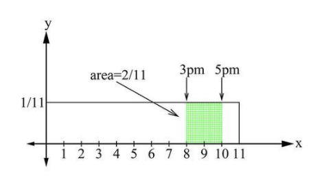
But, mathematically, how does the above calculation standup when the 11-hour interval and the 2-hour interval contain an infinite number of times? How can one infinitydivided by another infinity produce a probability of 0.182? (Note: The possible delivery times in the 11-hour interval represent a continuous random variable.) To resolve this issue, we can represent the probability of delivery of the package at any time in the 11-hour interval as being defined by a rectangle of height \( \frac{1}{11} \nonumber\) and length 11, with resulting area equal to 1. Looking at the 2-hour interval, we can see that it is equal to \( \frac{2}{11} \nonumber\) of the total rectangular area of 1. This is why it is therefore convenient to represent probabilities as areas.

Since areas can be defined by definite integrals, we can also define the probability of an event occuring within an interval [a, b] by the definite integral \( P(a≤x≤b)=\int\limits_a^b f(x)dx \nonumber\) where f(x) is called the probability density function (pdf).

A function f(x) is called a probability density function if

1. f(x)≥0 for all x
2. The area under the graph of f(x) over all the real line is exactly 1
3. The probability that x is in the interval [a, b] is

\[ P(a≤x≤b)=\int\limits_a^b f(x)dx \nonumber\]

i.e., the area under the graph of f(x) from a to b.

In the problem above, the probability density function f(x) is called a uniform (flat) probability density function (pdf).

Many other probability density functions exist that when used would give a different answer to the question about the delivery time of our package.

Suppose that after some thought and discussion with neighbors, you decide that it would be better to use a triangular probability density function as shown below for package delivery in your area. What is the probability that you will receive your package sometime between 3:00 PM and 5:00 PM?

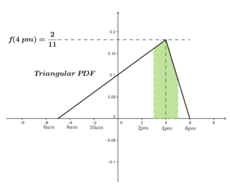
The triangular pdf shows a variation that can be modeled as:

\[ f(x)= \begin{cases} \frac{2}{99} (x+12) − \frac{14}{99}, −5 ≤ x ≤ 4 \\ \frac{−1}{11} (x+12)+ \frac{18}{11}, 4≤x≤6 \end{cases} \nonumber\]

Note that the pdf is 0 outside the above interval.

The probability that the package will arrive between 3 and 5 pm can be determined as

\( P(a≤x≤b)=\int\limits_a^b f(x)dx \nonumber\)

\( P(3≤x≤5)=\int\limits_3^5 f(x)dx \nonumber\)

\( = \int\limits_3^4 (\frac{2}{99} (x+12)− \frac{14}{99})dx+\int\limits_4^5 −\frac{1}{11} (x+12)−\frac{18}{11})dx \nonumber\)

\( =\frac{2}{99}[\frac{x^2}{2}+5x]_3^4−\frac{1}{11}[\frac{x^2}{2}−6x]_4^5 \nonumber\)

\( =\frac{17}{99}+\frac{1.5}{11} \nonumber\)

\( P(3≤x≤5)=\frac{30.5}{99}≈0.308 \nonumber\)

Using the triangular pdf, the probability of receiving the package between 3 and 5 pm has increased to 0.308.

The Normal Probability Density Function

One of the most useful probability density functions is the normal or Gaussian probability density function (sometimes referred to as the bell curve) defined as:

The Gaussian curve for a population with mean μ and standard deviation σ is given by \( f(x)=\frac{1}{σ\sqrt{2π}} e^{\frac{−(x−μ)^2}{(2σ2)}} \nonumber\), where the factor \( \frac{1}{(σ\sqrt{2π})} \nonumber\) is called the normalization constant, which is needed to make the probability over the entire space equal to 1.

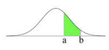
The density function has the bell curve shape represented below:

This function enables us to describe an entire population based on statistical measurements taken from a small sample of the population. The only measurements needed are the mean (μ) and the standard deviation (σ). Once those two numbers are known, the normal curve is defined.

Suppose that boxes containing 100 tea bags have a mean weight of 10.2 ounces each and a standard deviation of 0.1 ounce. What percentage of all the boxes is expected to weigh between 10 and 10.5 ounces? What is the probability that a box weighs less than 10 ounces? What is the probability that a box will weigh exactly 10 ounces?

Using the normal probability density function, \( f(x)=\frac{1}{σ\sqrt{2π}} e^{\frac{−(x−μ)^2}{(2σ^2)}} \nonumber\).

Substituting for μ=10.2 and σ=0.1, we get

\[ f(x)=\frac{1}{(0.1)\sqrt{2π}} e^{\frac{−(x−10.2)^2}{(2(0.1)^2)}} \nonumber\].

The percentage of all the tea boxes that are expected to weight between 10 and 10.5 ounces can be calculated as

\( P(10≤x≤10.5) = \int\limits_10^10.5 \frac{1}{(0.1) \sqrt{2π}} e^{\frac{−(x−10.2)^2}{(2(0.1)^2)}} dx \nonumber\).

The integral of \( e^{x^2} \nonumber\) does not have an elementary anti-derivative and therefore cannot be evaluated by standard techniques. However, we can use numerical techniques, such as The Simpson’s Rule or The Trapezoid Rule, to find an approximate (but very accurate) value. Using the programming feature of a scientific calculator or, mathematical software, we eventually get

\( \int\limits_{10}^{10.51} \frac{1}{(0.1)\sqrt{2π}} e^{\frac{−(x−10.2)^2}{(2(0.1)^2)}}dx≈0.976 \mbox{ That is, } P(10≤x≤10.5)≈0.976 \nonumber\).

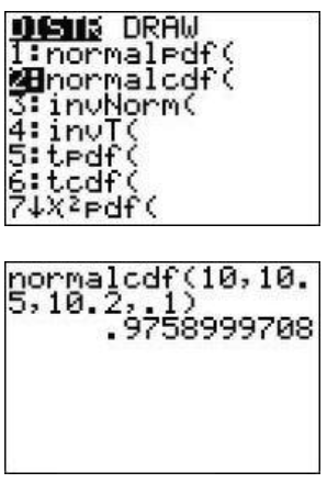
Technology Note: To make this computation with a graphing calculator of the TI-83/84 family, do the following:

From the [DISTR] menu (Figure 6.11.4) select option 2, which puts the phrase “normalcdf” in the home screen. Add lower bound, upper bound, mean, standard deviation, separated by commas, close the parentheses, and press [ENTER]. The result is shown in Figure 6.11.5.

For the probability that a box weighs less than 10.2 ounces, we use the area under the curve to the left of x=10.2.

Integrating numerically, we get

\[ P(9≤x≤10) = \int\limits_9^{10} \frac{1}{(0.1)\sqrt{2π}} e^{\frac{−(x−10.2)^2}{(2(0.1)^2)}} dx \nonumber\]

\[ P(9≤x≤10.2)≈0.02275 \nonumber\]

\[=2.28%, \nonumber\]

which says that we would expect 2.28% of the boxes to weigh less than 10 ounces.

Theoretically the probability here will be exactly zero because we will be integrating from 10 to 10 which is zero. However, since all scales have some error (call it ϵ), practically we would find the probability that the weight falls between 10−ϵ and 10+ϵ.

---

Examples

Example 1

Earlier, you were asked to determine which type of random variable (discrete or continuous) would be associated with probabilities computed using definite integrals.

If you said that the continuous random variable would be associated with probabilities determined by definite integrals, you would be correct.

Example 2

An Intelligence Quotient or IQ is a score derived from different standardized tests attempting to measure the level of intelligence of an adult human being. The average score of the test is 100 and the standard deviation is 15. What is the percentage of the population that has a score between 85 and 115? What percentage of the population has a score above 140?

Using the normal probability density function, \( f(x) = \frac{1}{σ \sqrt{2π}}  e^{ \frac{−(x−μ)^2}{(2σ^2)}} \nonumber\), 

and substituting \( μ=100 \mbox{ and } σ=15, f(x)= \frac{1}{15\sqrt{2π}}e^{\frac{−(x−100)^2}{(2(15)^2)}} \nonumber\).

The percentage of the population that has a score between 85 and 115 is \( P(85≤x≤115)= \int\limits_85^115 \frac{1}{15\sqrt{2π}} e^{ \frac{−(x−100)^2}{(2(15)^2)}} \nonumber\).

Again, the integral of \( e^{−x^2} \nonumber\) does not have an elementary anti-derivative and therefore cannot be evaluated. Using the programming feature of a scientific calculator or a mathematical computer software, we get \( \int\limits_85^115 \frac{1}{15\sqrt{2π}}e^{−(x−100)^2}{(2(15)^2)} dx≈0.68 \nonumber\). That is, \( P(85≤x≤115)≈68% \nonumber\)

Which says that 68% of the population has an IQ score between 85 and 115.

To measure the probability that a person selected randomly will have an IQ score above 140, \( P(x≥140)= \int\limits_{140}^\infty \frac{1}{15\sqrt{2π}}e^{\frac{−(x−100)^2}{(2(15)^2)}} dx \nonumber\)

This integral is even more difficult to integrate since it is an improper integral. To avoid the messy work, we can argue that since it is extremely rare to meet someone with an IQ score of over 200 we can approximate the integral from 140 to 200 Then

\( P(x≥140) = \int\limits_{140}^{200} \frac{1}{15\sqrt{2π}}e^{\frac{−(x−100)^2}{(2(15)^2)}} dx \nonumber\)

Integrating numerically, we get P(x≥140)≈0.0039.

So the probability of selecting at random a person with an IQ score above 140 is 0.0039. That’s about one person in every 250 individuals!

---

Review

For #1-4, find the number r that makes the function a probability density function over the given sample space.

1. \( f(x)=r \nonumber\) over the sample space of [-7, 7].
2. \( f(x)=rx(x−5) \nonumber\) over the sample space of [0, 5].
3. \( f(x)= \frac{r}{(1+x)^2} \nonumber\) over the sample space of [0, 25].
4. \( f(x)=rsinx \nonumber\) over the sample space of \( [0, \frac{π}{2}] \nonumber\).
5. Given a triangular probability density function g(x) over the sample space [0, 10], what is the highest value of g(x) if it occurs at x=7?
6. Could the function \( g(x)=\frac{−4}{25}x+0.9 \nonumber\) be a probability density function over the interval [0, 10]?
7. Suppose f(x) is the probability density function for the lifetime of a manufacturer’s light bulb, where x is measured in hours. Explain the meaning of each integral.
   1. \( \int_1000^5000 f(x)dx \nonumber\)
   2. \( \int_3000^∞ f(x)dx \nonumber\)
8. Suppose \( f(x)=−\frac{1}{36}(x^2−9) \nonumber\) is the probability density function for an event’s time of occurrence within the time window [-3, +3 hours] (0 is on time occurrence). What is the probability the event occurs within ±1 hour of the expected time?
9. For problem #8, what time window guarantees a 90% probability of occurrence?
10. The length of time a customer spends waiting until his/her entree is served at a certain restaurant is modeled by an exponential density function \( f(x)=0.125e^{−0.125t} \nonumber\), where \( \frac{1}{0.125}=8\nonumber\) is the average wait time in minutes.
    1. What is the probability that a customer is served in the first 3 minutes?
    2. What is the probability that a customer has to wait more than 10 minutes?
11. The average height of an adult female in Los Angeles is 63.4 inches (5 feet, 3.4 inches) with a standard deviation of 3.2 inches.
    1. What is the probability that a female’s height is less than 63.4 inches?
    2. What is the probability that a female’s height is between 63 and 65 inches?
    3. What is the probability that a female’s height is more than 6 feet?
    4. What is the probability that a female’s height is exactly 5 feet?
    5. The median of a distribution with a probability density function f(x), is the value M such that \( \int_{-∞}^M f(x)dx=0.5 \nonumber\). Half the values of the distribution will be above M, and half will be below M. Find the median value for each of the following probability density functions:
12. \( f(x)=−\frac{1}{36} (x^2−9) \nonumber\) over the interval [-3, 3].
13. \( f(x)=0.125e^{−0.125t} \nonumber\) over the interval [0, ∞).
    1. The mean of a distribution with the probability density function f(x), is the value given by \( \int_{−∞}^∞ xf(x)dx \nonumber\). Find the mean value for each of the following probability density functions:
14. \( f(x)=−\frac{1}{36}(x^2−9) \nonumber\) over the interval [-3, 3].
15. \( f(x)=0.125e^{−0.125t}  \nonumber\) over the interval [0, ∞).

---

Review (Answers)

To see the Review answers, open this PDF file and look for section 6.10.

---

Vocabulary

Term	Definition
Gaussian probability density function	A Normal (Gaussian) pdf is a continuous pdf defined by f(x)=1σ2π√e−(x−μ)2(2σ2) where μ is the mean, and σ is the standard deviation.
mean	The mean of a distribution with the probability density function f(x) is the value given by ∫−∞∞xf(x)dx.
median	The median of a distribution with a probability density function f(x) is the value M such that ∫−∞Mf(x)dx=0.5. Half the values of the distribution will be above M, and half will be below M.
normal probability density function	A Normal (Gaussian) pdf is a continuous pdf defined by f(x)=1σ2π√e−(x−μ)2(2σ2) where μ is the mean, and σ is the standard deviation.
pdf	A function f(x) is called a probability density function (pdf) if f(x)≥0 for all x, the area under the graph of f(x) over all real numbers is exactly 1, and the probability that x is in the interval [a, b] is P(a≤x≤b)=∫abf(x)dx.
Probability	Probability is the chance that something will happen. It can be written as a fraction, decimal or percent.
probability density function	A function f(x) is called a probability density function if f(x)≥0 for all x, the area under the graph of f(x) over all real numbers is exactly 1, and the probability that x is in the interval [a, b] is P(a≤x≤b)=∫abf(x)dx.
triangular probability density function	A triangular probability density function (pdf) is a continuous pdf whose triangular shape is defined by three values of x : a lower value, a mode value with highest distribution value, and an upper value.
uniform probability density function	A uniform (or rectangular, flat) probability density function (pdf) P(x) is a continuous distribution where every equal interval of x has the same probability.

---

Additional Resources

Video: More on Probability Density Functions

Real World: Preventable Deaths