
9.5: Trapezoidal and Midpoint Approximations
- Page ID
- 1254
\( \newcommand{\vecs}[1]{\overset { \scriptstyle \rightharpoonup} {\mathbf{#1}} } \)
\( \newcommand{\vecd}[1]{\overset{-\!-\!\rightharpoonup}{\vphantom{a}\smash {#1}}} \)
\( \newcommand{\dsum}{\displaystyle\sum\limits} \)
\( \newcommand{\dint}{\displaystyle\int\limits} \)
\( \newcommand{\dlim}{\displaystyle\lim\limits} \)
\( \newcommand{\id}{\mathrm{id}}\) \( \newcommand{\Span}{\mathrm{span}}\)
( \newcommand{\kernel}{\mathrm{null}\,}\) \( \newcommand{\range}{\mathrm{range}\,}\)
\( \newcommand{\RealPart}{\mathrm{Re}}\) \( \newcommand{\ImaginaryPart}{\mathrm{Im}}\)
\( \newcommand{\Argument}{\mathrm{Arg}}\) \( \newcommand{\norm}[1]{\| #1 \|}\)
\( \newcommand{\inner}[2]{\langle #1, #2 \rangle}\)
\( \newcommand{\Span}{\mathrm{span}}\)
\( \newcommand{\id}{\mathrm{id}}\)
\( \newcommand{\Span}{\mathrm{span}}\)
\( \newcommand{\kernel}{\mathrm{null}\,}\)
\( \newcommand{\range}{\mathrm{range}\,}\)
\( \newcommand{\RealPart}{\mathrm{Re}}\)
\( \newcommand{\ImaginaryPart}{\mathrm{Im}}\)
\( \newcommand{\Argument}{\mathrm{Arg}}\)
\( \newcommand{\norm}[1]{\| #1 \|}\)
\( \newcommand{\inner}[2]{\langle #1, #2 \rangle}\)
\( \newcommand{\Span}{\mathrm{span}}\) \( \newcommand{\AA}{\unicode[.8,0]{x212B}}\)
\( \newcommand{\vectorA}[1]{\vec{#1}} % arrow\)
\( \newcommand{\vectorAt}[1]{\vec{\text{#1}}} % arrow\)
\( \newcommand{\vectorB}[1]{\overset { \scriptstyle \rightharpoonup} {\mathbf{#1}} } \)
\( \newcommand{\vectorC}[1]{\textbf{#1}} \)
\( \newcommand{\vectorD}[1]{\overrightarrow{#1}} \)
\( \newcommand{\vectorDt}[1]{\overrightarrow{\text{#1}}} \)
\( \newcommand{\vectE}[1]{\overset{-\!-\!\rightharpoonup}{\vphantom{a}\smash{\mathbf {#1}}}} \)
\( \newcommand{\vecs}[1]{\overset { \scriptstyle \rightharpoonup} {\mathbf{#1}} } \)
\(\newcommand{\longvect}{\overrightarrow}\)
\( \newcommand{\vecd}[1]{\overset{-\!-\!\rightharpoonup}{\vphantom{a}\smash {#1}}} \)
\(\newcommand{\avec}{\mathbf a}\) \(\newcommand{\bvec}{\mathbf b}\) \(\newcommand{\cvec}{\mathbf c}\) \(\newcommand{\dvec}{\mathbf d}\) \(\newcommand{\dtil}{\widetilde{\mathbf d}}\) \(\newcommand{\evec}{\mathbf e}\) \(\newcommand{\fvec}{\mathbf f}\) \(\newcommand{\nvec}{\mathbf n}\) \(\newcommand{\pvec}{\mathbf p}\) \(\newcommand{\qvec}{\mathbf q}\) \(\newcommand{\svec}{\mathbf s}\) \(\newcommand{\tvec}{\mathbf t}\) \(\newcommand{\uvec}{\mathbf u}\) \(\newcommand{\vvec}{\mathbf v}\) \(\newcommand{\wvec}{\mathbf w}\) \(\newcommand{\xvec}{\mathbf x}\) \(\newcommand{\yvec}{\mathbf y}\) \(\newcommand{\zvec}{\mathbf z}\) \(\newcommand{\rvec}{\mathbf r}\) \(\newcommand{\mvec}{\mathbf m}\) \(\newcommand{\zerovec}{\mathbf 0}\) \(\newcommand{\onevec}{\mathbf 1}\) \(\newcommand{\real}{\mathbb R}\) \(\newcommand{\twovec}[2]{\left[\begin{array}{r}#1 \\ #2 \end{array}\right]}\) \(\newcommand{\ctwovec}[2]{\left[\begin{array}{c}#1 \\ #2 \end{array}\right]}\) \(\newcommand{\threevec}[3]{\left[\begin{array}{r}#1 \\ #2 \\ #3 \end{array}\right]}\) \(\newcommand{\cthreevec}[3]{\left[\begin{array}{c}#1 \\ #2 \\ #3 \end{array}\right]}\) \(\newcommand{\fourvec}[4]{\left[\begin{array}{r}#1 \\ #2 \\ #3 \\ #4 \end{array}\right]}\) \(\newcommand{\cfourvec}[4]{\left[\begin{array}{c}#1 \\ #2 \\ #3 \\ #4 \end{array}\right]}\) \(\newcommand{\fivevec}[5]{\left[\begin{array}{r}#1 \\ #2 \\ #3 \\ #4 \\ #5 \\ \end{array}\right]}\) \(\newcommand{\cfivevec}[5]{\left[\begin{array}{c}#1 \\ #2 \\ #3 \\ #4 \\ #5 \\ \end{array}\right]}\) \(\newcommand{\mattwo}[4]{\left[\begin{array}{rr}#1 \amp #2 \\ #3 \amp #4 \\ \end{array}\right]}\) \(\newcommand{\laspan}[1]{\text{Span}\{#1\}}\) \(\newcommand{\bcal}{\cal B}\) \(\newcommand{\ccal}{\cal C}\) \(\newcommand{\scal}{\cal S}\) \(\newcommand{\wcal}{\cal W}\) \(\newcommand{\ecal}{\cal E}\) \(\newcommand{\coords}[2]{\left\{#1\right\}_{#2}}\) \(\newcommand{\gray}[1]{\color{gray}{#1}}\) \(\newcommand{\lgray}[1]{\color{lightgray}{#1}}\) \(\newcommand{\rank}{\operatorname{rank}}\) \(\newcommand{\row}{\text{Row}}\) \(\newcommand{\col}{\text{Col}}\) \(\renewcommand{\row}{\text{Row}}\) \(\newcommand{\nul}{\text{Nul}}\) \(\newcommand{\var}{\text{Var}}\) \(\newcommand{\corr}{\text{corr}}\) \(\newcommand{\len}[1]{\left|#1\right|}\) \(\newcommand{\bbar}{\overline{\bvec}}\) \(\newcommand{\bhat}{\widehat{\bvec}}\) \(\newcommand{\bperp}{\bvec^\perp}\) \(\newcommand{\xhat}{\widehat{\xvec}}\) \(\newcommand{\vhat}{\widehat{\vvec}}\) \(\newcommand{\uhat}{\widehat{\uvec}}\) \(\newcommand{\what}{\widehat{\wvec}}\) \(\newcommand{\Sighat}{\widehat{\Sigma}}\) \(\newcommand{\lt}{<}\) \(\newcommand{\gt}{>}\) \(\newcommand{\amp}{&}\) \(\definecolor{fillinmathshade}{gray}{0.9}\)Recall that we have used different ways to approximate the value of integrals. These included Riemann Sums using left and right endpoints, as well as midpoints for finding the length of each rectangular tile. In this lesson the rectangular tiles are replace by trapezoidal tiles to approximate the integral. Do you think that the use of trapezoids would give a more accurate result than the use of rectangles? Why? Can you think of a reason why the concavity of the function curve would matter in the accuracy of the area estimation using trapezoids?
Recall that we used different ways to approximate the value of integrals. These included Riemann Sums using left and right endpoints, as well as midpoints for finding the length of each rectangular tile. In this lesson we will learn two other methods for approximating integrals. The first of these, the Trapezoidal Rule, uses areas of trapezoidal tiles to approximate the integral. The second method, Simpson’s Rule, uses parabolas to make the approximation.
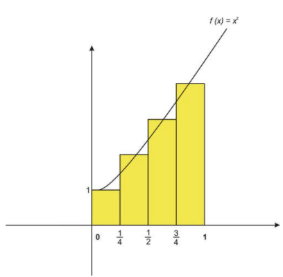
Let’s recall how we would use the midpoint rule with n=4 rectangles to approximate the area under the graph of \( f(x)=x^2+1 \nonumber\) from x=0 to x=1.
CC BY-NC-SA
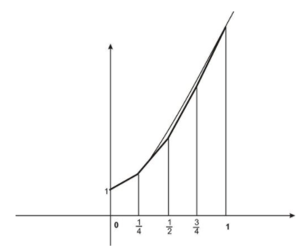
If instead of using the midpoint value within each sub-interval to find the length of the corresponding rectangle, we could have instead formed trapezoids by joining the maximum and minimum values of the function within each sub-interval:
CC BY-NC-SA
The area of a trapezoid is \( A= \frac{h(b_1+b_2)}{2} \nonumber\), where b1 and b2 are the lengths of the parallel sides and h is the height. In our trapezoids the height is △x and b1 and b2 are the values of the function. Therefore in finding the areas of the trapezoids we actually average the left and right endpoints of each sub-interval.
Therefore a typical trapezoid would have the area
\[ A = \frac{△x}{2} (f(x_{i−1})+f(x_i)) \nonumber\].
To approximate \( \int\limits_a^b f(x)dx with n of these trapezoids, we have
\[ \int\limits_a^b f(x)dx ≈ \frac{1}{2} [|\sum_{i=1}^n f(x_{i−1})△x+ \sum_{i=1}^n f(x_i)△x] \nonumber\]
\[ = \frac{△x}{2} [f(x_0)+f(x_1)+f(x_1)+f(x_2)+f(x_2)+⋯+f(x_{n−1})+f(x_n)] \nonumber\]
\[ = \frac{△x}{2} [f(x_0)+2f(x_1)+2f(x_2)+⋯+2f(x_{n−1})+f(x_n)],△x= \frac{b−a}{n} \nonumber\].
Apply the formula from above and use the Trapezoidal Rule to approximate \( \int\limits_0^3 x^2dx \nonumber\) with n=6.
Each subinterval is \( △x= \frac{b−a}{n}= \frac{3−0}{6}= \frac{1}{2} \nonumber\).
The integral approximation is:
\[ \int\limits_0^3 x^2 dx ≈ \frac{1}{4} [f(0)+2f( \frac{1}{2})+ 2 f (1)+ 2 f ( \frac{3}{2})+2f(2)+2f( \frac{5}{2})+f(3)] \nonumber\]
\[ = \frac{1}{4} [0+(2⋅ \frac{1}{4})+(2⋅1)+(2⋅ \frac{9}{4})+(2⋅4)+(2⋅ \frac{25}{4} )+9] \nonumber\]
\[ = \frac{1}{4} [ \frac{73}{2}]= \frac{73}{8} = 9.125. \nonumber\]
An exact solution can be determined by using the antiderivative with the Fundamental Theorem.
\[ \int\limits_0^3 x^2 dx = \frac{x^3}{3} |_0^3 = 9 . \nonumber\]
The error is about 1.4%.
For some integrals it is impossible to find an antiderivative and a numerical method is the only option.
When this is the case, accuracy of the approximation is an issue. In particular, how large should n be so that the trapezoidal estimate is accurate to within a given value, say 0.001?
The magnitude of the error in using the trapezoidal technique for a given value of n can be shown to be:
\[ |Error_{Trapezoidal} | ≤ \frac{k(b−a)^3}{12 n^2}, \mbox{ where } |f′′(x)|≤k \mbox{ for } a≤x≤b \nonumber\]
This means that choosing \( n ≥ \sqrt{ \frac{k(b−a)^3}{12} ⋅ |Error_{Trapezoidal}| } \nonumber\) will meet or exceed a specified error ErrorTrapezoidal.
Find n so that the Trapezoidal Estimate for \( \int_0^3 x^2 dx \nonumber\) is accurate to 0.001.
We need to find n such that \( |Error_{Trapezoidal}| ≤ 0.001 \nonumber\).
First note that \( |f′′(x)|=2 \mbox{ for } 0≤x≤3 \nonumber\). Hence we can take k=2 to find our error bound.
\[ |Error_{Trapezoidal}| ≤ \frac{2 (3−0)^3}{12 n^2} = \frac{54}{12 n^2} \nonumber\]
We need to solve the following inequality for n:
\[ \frac{54}{12n^2} < 0.001, \nonumber\]
\[ n^2 > \frac {54}{12(0.001)}, \nonumber\]
\[ n > \sqrt{ \frac{54}{12(0.001)}} ≈ 67.08 \nonumber\]
Hence we must take n=68 to achieve the desired accuracy.
Examples
Example 1
Earlier, you were asked if you think that using trapezoids to approximate the area under a curve would give a more accurate result than using rectangles. Can you think of a reason why the concavity of the function curve would matter in the accuracy of the area estimation using trapezoids?
If you think that the use of trapezoids would give a more accurate result (with number of subintervals the same) you are correct. With some examples, you can see visually that the trapezoids cover the area under the curve better. Notice, though, that if the function curve is concave up, the trapezoids will overestimate the area; if the concavity is down, the trapezoids will underestimate the area.
Example 2
Use the Trapezoidal Rule to approximate ∫02x3dx for n=4. Round the answer to four decimal places and compare this value to the exact value of the integral. What is the expected error for n=4?
We find each subinterval as △x=b−an=2−04=12.
The integral approximation is evaluated as follows:
\[ \int\limits_0^2 x^3 dx ≈ \frac{1}{4} [f(0) + 2 f(0.5) + 2 f(1) + 2 f(1.5) + f(2) ] \nonumber\]
\[ ≈ \frac{1}{4} [0+2⋅0.125+2⋅1+2⋅3.375+8] \nonumber\]
\[ \int\limits_0^2 x^3 dx ≈ 4.25 \nonumber\]
The estimate of the integral is 4.25.
The exact value of the integral: \( \int\limits_0^2 x^3 dx = \frac{x^4}{4}|_0^2 = 4 \nonumber\).
The error between these is 0.25.
The expected error using n=4:
For f′′(x)=6x, f′′(x)≤6⋅2=12 in the interval [0,2].
Therefore, \( |Error_{Trapezoidal}| ≤ \frac{k(b−a)^3}{12 n^2} = \frac{12(2)^3}{12⋅4^2}=0.5 \nonumber\).
The actual error is less than \( |Error_{Trapezoidal}| \nonumber\).
Example 3
Use the Trapezoidal Rule to approximate \( \int\lim_1^2 \frac{1}{(x+1)^2} dx \nonumber\) for n=4. Round the answer to four decimal places and compare this value to the exact value of the integral. What is the expected error for n=4?
We find each subinterval as \( △x = \frac{b−a}{n} = \frac{2−1}{4} = \frac{1}{4} \nonumber\).
The integral approximation is evaluated as follows:
\[ \int\limits_1^2 \frac{1}{(x+1)^2} dx ≈ \frac{1}{8} [f(2)+2f(2.25)+2f(2.5)+2f(2.75)+f(3)] \nonumber\]
\[ ≈ \frac{1}{8} [\frac{1}{4} + 2 \frac{1}{2.25^2} + 2 \frac{1}{2.5^2} + 2 \frac{1}{2.75^2} + \frac{1}{3^2} ] \nonumber\]
\[ ≈ \frac{1}{8} [0.25+0.39506+0.32+0.26446+0.11111] \nonumber\]
\[ \int\limits_1^2 \frac{1}{(x+1)^2} dx ≈ 0.16758 ≈ 0.1676 \nonumber\]
The estimate of the integral is 0.1676.
The exact value of the integral: \[ ∫121(x+1)2dx=−1x+1∣∣∣21=16=0.16⎯⎯⎯ \nonumber\].
The error between these is 0.0009.
The expected error using n=4:
For \( f′′(x) = \frac{6}{(x+1)^4}, f′′(x) ≤ \frac{6}{(1+1)^4} = \frac{3}{8} = 0.375 \nonumber\) in the interval [1, 2].
Therefore, \(|Error_{Tropezoidal}| ≤ \frac{k(b−a)^3}{12n^2} = \frac{0.375(1)^3}{12⋅4^2} = 0.001953 \nonumber\).
The actual error is less than \( |Error_{Trapeziodal}| \nonumber\).
Review
Use the Trapezoidal Rule to approximate the definite integrals using the given number of subintervals n.
- \( \int_1^7 (x+7)dx \mbox{ with } n=6 \nonumber\).
- \( \int_{−2}^2 (x+4)dx \mbox{ with } n=4 \nonumber\).
- \( \int_{−4}{1} (−x^2−2x+8) dx \mbox{ with } n=5 \nonumber\).
- \( \int_2^7 \frac{2}{x} dx \mbox{ with } n=5 \nonumber\).
- \( \int_0^2 x^4 dx \mbox{ with } n=4 \nonumber\).
- \( \int_0^1 sin \frac{x}{2} dx \mbox{ with } n=4 \nonumber\).
- \( \int_2^4 \sqrt{x} dx \mbox{ with } n=5 \nonumber\).
- \( \int_0^1 x^2e−xdx \mbox{ with } n=8 \nonumber\).
- \( \int_1^4 ln\sqrt{x} dx \mbox{ with } n=6 \nonumber\).
- \( \int_0^1 \sqrt{1+x^4}dx \mbox{ with } n=4 \nonumber\).
- \( \int_1^3 \frac{1}{x} dx \mbox{ with } n=8 \nonumber\).
- \( \int_0^2 x^3 dx \mbox{ for } n=8 \nonumber\) .
- Find a value of n that guarantees an error of no more than 10−5 in the Trapezoidal approximation of \( \int_2^4 \sqrt{x} dx \nonumber\). How large should n be so that the Trapezoidal Estimate for \( \int_1^3 \frac{1}{x} dx \nonumber\) is accurate to within:
- 0.001?
- 0.00001?
Vocabulary
| Term | Definition |
|---|---|
| trapezoidal rule | The trapezoidal rule is a method for computing a definite integral by computing the area trapezoidal segments in the integration interval and summing them. |
Additional Resources
PLIX: Play, Learn, Interact, eXplore - Area of a Skirt
Video: Trapezoid Approximation of Area Under Curve by Khan Academy
Practice: Trapezoidal and Midpoint Approximations