1.3: Introduction to Data and Measurement Issues
- Page ID
- 5693
\( \newcommand{\vecs}[1]{\overset { \scriptstyle \rightharpoonup} {\mathbf{#1}} } \)
\( \newcommand{\vecd}[1]{\overset{-\!-\!\rightharpoonup}{\vphantom{a}\smash {#1}}} \)
\( \newcommand{\id}{\mathrm{id}}\) \( \newcommand{\Span}{\mathrm{span}}\)
( \newcommand{\kernel}{\mathrm{null}\,}\) \( \newcommand{\range}{\mathrm{range}\,}\)
\( \newcommand{\RealPart}{\mathrm{Re}}\) \( \newcommand{\ImaginaryPart}{\mathrm{Im}}\)
\( \newcommand{\Argument}{\mathrm{Arg}}\) \( \newcommand{\norm}[1]{\| #1 \|}\)
\( \newcommand{\inner}[2]{\langle #1, #2 \rangle}\)
\( \newcommand{\Span}{\mathrm{span}}\)
\( \newcommand{\id}{\mathrm{id}}\)
\( \newcommand{\Span}{\mathrm{span}}\)
\( \newcommand{\kernel}{\mathrm{null}\,}\)
\( \newcommand{\range}{\mathrm{range}\,}\)
\( \newcommand{\RealPart}{\mathrm{Re}}\)
\( \newcommand{\ImaginaryPart}{\mathrm{Im}}\)
\( \newcommand{\Argument}{\mathrm{Arg}}\)
\( \newcommand{\norm}[1]{\| #1 \|}\)
\( \newcommand{\inner}[2]{\langle #1, #2 \rangle}\)
\( \newcommand{\Span}{\mathrm{span}}\) \( \newcommand{\AA}{\unicode[.8,0]{x212B}}\)
\( \newcommand{\vectorA}[1]{\vec{#1}} % arrow\)
\( \newcommand{\vectorAt}[1]{\vec{\text{#1}}} % arrow\)
\( \newcommand{\vectorB}[1]{\overset { \scriptstyle \rightharpoonup} {\mathbf{#1}} } \)
\( \newcommand{\vectorC}[1]{\textbf{#1}} \)
\( \newcommand{\vectorD}[1]{\overrightarrow{#1}} \)
\( \newcommand{\vectorDt}[1]{\overrightarrow{\text{#1}}} \)
\( \newcommand{\vectE}[1]{\overset{-\!-\!\rightharpoonup}{\vphantom{a}\smash{\mathbf {#1}}}} \)
\( \newcommand{\vecs}[1]{\overset { \scriptstyle \rightharpoonup} {\mathbf{#1}} } \)
\( \newcommand{\vecd}[1]{\overset{-\!-\!\rightharpoonup}{\vphantom{a}\smash {#1}}} \)
\(\newcommand{\avec}{\mathbf a}\) \(\newcommand{\bvec}{\mathbf b}\) \(\newcommand{\cvec}{\mathbf c}\) \(\newcommand{\dvec}{\mathbf d}\) \(\newcommand{\dtil}{\widetilde{\mathbf d}}\) \(\newcommand{\evec}{\mathbf e}\) \(\newcommand{\fvec}{\mathbf f}\) \(\newcommand{\nvec}{\mathbf n}\) \(\newcommand{\pvec}{\mathbf p}\) \(\newcommand{\qvec}{\mathbf q}\) \(\newcommand{\svec}{\mathbf s}\) \(\newcommand{\tvec}{\mathbf t}\) \(\newcommand{\uvec}{\mathbf u}\) \(\newcommand{\vvec}{\mathbf v}\) \(\newcommand{\wvec}{\mathbf w}\) \(\newcommand{\xvec}{\mathbf x}\) \(\newcommand{\yvec}{\mathbf y}\) \(\newcommand{\zvec}{\mathbf z}\) \(\newcommand{\rvec}{\mathbf r}\) \(\newcommand{\mvec}{\mathbf m}\) \(\newcommand{\zerovec}{\mathbf 0}\) \(\newcommand{\onevec}{\mathbf 1}\) \(\newcommand{\real}{\mathbb R}\) \(\newcommand{\twovec}[2]{\left[\begin{array}{r}#1 \\ #2 \end{array}\right]}\) \(\newcommand{\ctwovec}[2]{\left[\begin{array}{c}#1 \\ #2 \end{array}\right]}\) \(\newcommand{\threevec}[3]{\left[\begin{array}{r}#1 \\ #2 \\ #3 \end{array}\right]}\) \(\newcommand{\cthreevec}[3]{\left[\begin{array}{c}#1 \\ #2 \\ #3 \end{array}\right]}\) \(\newcommand{\fourvec}[4]{\left[\begin{array}{r}#1 \\ #2 \\ #3 \\ #4 \end{array}\right]}\) \(\newcommand{\cfourvec}[4]{\left[\begin{array}{c}#1 \\ #2 \\ #3 \\ #4 \end{array}\right]}\) \(\newcommand{\fivevec}[5]{\left[\begin{array}{r}#1 \\ #2 \\ #3 \\ #4 \\ #5 \\ \end{array}\right]}\) \(\newcommand{\cfivevec}[5]{\left[\begin{array}{c}#1 \\ #2 \\ #3 \\ #4 \\ #5 \\ \end{array}\right]}\) \(\newcommand{\mattwo}[4]{\left[\begin{array}{rr}#1 \amp #2 \\ #3 \amp #4 \\ \end{array}\right]}\) \(\newcommand{\laspan}[1]{\text{Span}\{#1\}}\) \(\newcommand{\bcal}{\cal B}\) \(\newcommand{\ccal}{\cal C}\) \(\newcommand{\scal}{\cal S}\) \(\newcommand{\wcal}{\cal W}\) \(\newcommand{\ecal}{\cal E}\) \(\newcommand{\coords}[2]{\left\{#1\right\}_{#2}}\) \(\newcommand{\gray}[1]{\color{gray}{#1}}\) \(\newcommand{\lgray}[1]{\color{lightgray}{#1}}\) \(\newcommand{\rank}{\operatorname{rank}}\) \(\newcommand{\row}{\text{Row}}\) \(\newcommand{\col}{\text{Col}}\) \(\renewcommand{\row}{\text{Row}}\) \(\newcommand{\nul}{\text{Nul}}\) \(\newcommand{\var}{\text{Var}}\) \(\newcommand{\corr}{\text{corr}}\) \(\newcommand{\len}[1]{\left|#1\right|}\) \(\newcommand{\bbar}{\overline{\bvec}}\) \(\newcommand{\bhat}{\widehat{\bvec}}\) \(\newcommand{\bperp}{\bvec^\perp}\) \(\newcommand{\xhat}{\widehat{\xvec}}\) \(\newcommand{\vhat}{\widehat{\vvec}}\) \(\newcommand{\uhat}{\widehat{\uvec}}\) \(\newcommand{\what}{\widehat{\wvec}}\) \(\newcommand{\Sighat}{\widehat{\Sigma}}\) \(\newcommand{\lt}{<}\) \(\newcommand{\gt}{>}\) \(\newcommand{\amp}{&}\) \(\definecolor{fillinmathshade}{gray}{0.9}\)The Galapagos Tortoises
In order to learn some basic vocabulary of statistics and learn how to distinguish between different types of variables, we will use the example of information about the Giant Galapagos Tortoise.

Approximating the Distribution of the Galapagos Tortoises
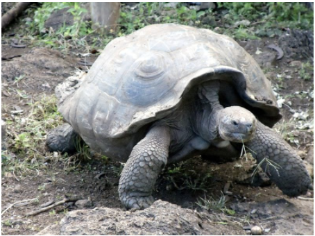
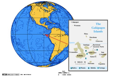
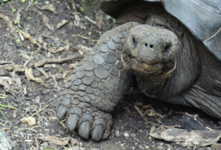
The Galapagos Islands, off the coast of Ecuador in South America, are famous for the amazing diversity and uniqueness of life they possess. One of the most famous Galapagos residents is the Galapagos Giant Tortoise, which is found nowhere else on earth. Charles Darwin’s visit to the islands in the 19th Century and his observations of the tortoises were extremely important in the development of his theory of evolution.

The tortoises lived on nine of the Galapagos Islands, and each island developed its own unique species of tortoise. In fact, on the largest island, there are four volcanoes, and each volcano has its own species. When first discovered, it was estimated that the tortoise population of the islands was around 250,000. Unfortunately, once European ships and settlers started arriving, those numbers began to plummet. Because the tortoises could survive for long periods of time without food or water, expeditions would stop at the islands and take the tortoises to sustain their crews with fresh meat and other supplies for the long voyages. Also, settlers brought in domesticated animals like goats and pigs that destroyed the tortoises' habitat. Today, two of the islands have lost their species, a third island has no remaining tortoises in the wild, and the total tortoise population is estimated to be around 15,000. The good news is there have been massive efforts to protect the tortoises. Extensive programs to eliminate the threats to their habitat, as well as breed and reintroduce populations into the wild, have shown some promise.
Approximate distribution of Giant Galapagos Tortoises in 2004, Estado Actual De Las Poblaciones de Tortugas Terrestres Gigantes en las Islas Galápagos, Marquez, Wiedenfeld, Snell, Fritts, MacFarland, Tapia, y Nanjoa, Scologia Aplicada, Vol. 3, Num. 1,2, pp. 98 11.
| Island or Volcano | Species | Climate Type | Shell Shape | Estimate of Total Population | Population Density (per km2) | Number of Individuals Repatriated∗ |
|---|---|---|---|---|---|---|
| Wolf | becki | semi-arid | intermediate | 1139 | 228 | 40 |
| Darwin | microphyes | semi-arid | dome | 818 | 205 | 0 |
| Alcedo | vanden- burghi | humid | dome | 6,320 | 799 | 0 |
| Sierra Negra | guntheri | humid | flat | 694 | 122 | 286 |
| Cerro Azul | vicina | humid | dome | 2.574 | 155 | 357 |
| Santa Cruz | nigrita | humid | dome | 3,391 | 730 | 210 |
| Española | hoodensis | arid | saddle | 869 | 200 | 1,293 |
| San Cristóbal | chathamen- sis | semi-arid | dome | 1,824 | 559 | 55 |
| Santiago | darwini | humid | intermediate | 1,165 | 124 | 498 |
| Pinzón | ephippium | arid | saddle | 532 | 134 | 552 |
| Pinta | abingdoni | arid | saddle | 1 | Does not apply | 0 |
∗Repatriation is the process of raising tortoises and releasing them into the wild when they are grown to avoid local predators that prey on the hatchlings.

Classifying Variables
Statisticians refer to an entire group that is being studied as a population. Each member of the population is called a unit. In this example, the population is all Galapagos Tortoises, and the units are the individual tortoises. It is not necessary for a population or the units to be living things, like tortoises or people. For example, an airline employee could be studying the population of jet planes in her company by studying individual planes.
A researcher studying Galapagos Tortoises would be interested in collecting information about different characteristics of the tortoises. Those characteristics are called variables. Each column of the previous figure contains a variable. In the first column, the tortoises are labeled according to the island (or volcano) where they live, and in the second column, by the scientific name for their species. When a characteristic can be neatly placed into well-defined groups, or categories, that do not depend on order, it is called a categorical variable, or qualitative variable.
The last three columns of the previous figure provide information in which the count, or quantity, of the characteristic is most important. We are interested in the total number of each species of tortoise, or how many individuals there are per square kilometer. This type of variable is called a numerical variable, or quantitative variable.
Determine whether each of the variables Climate Type, Shell Shape, Number of Tagged Individuals, and Number of Individuals Repatriated are numerical or categorical variables.
| Variable | Explanation | Type |
|---|---|---|
| Climate Type | Many of the islands and volcanic habitats have three distinct climate types. | Categorical |
| Shell Shape | Over many years, the different species of tortoises have developed different shaped shells as an adaptation to assist them in eating vegetation that varies in height from island to island. | Categorical |
| Number of Tagged Individuals | Tortoises were captured and marked by scientists to study their health and assist in estimating the total population. | Numerical |
| Number of Individuals Repatriated | There are two tortoise breeding centers on the islands. Through these programs, many tortoises have been raised and then reintroduced into the wild. | Numerical |
Population vs. Sample
We have already defined a population as the total group being studied. Most of the time, it is extremely difficult or very costly to collect all the information about a population. In the Galapagos, it would be very difficult and perhaps even destructive to search every square meter of the habitat to be sure that you counted every tortoise. In an example closer to home, it is very expensive to get accurate and complete information about all the residents of the United States to help effectively address the needs of a changing population. This is why a complete counting, or census, is only attempted every ten years. Because of these problems, it is common to use a smaller, representative group from the population, called a sample.
You may recall the tortoise data included a variable for the estimate of the population size. This number was found using a sample and is actually just an approximation of the true number of tortoises. If a researcher wanted to find an estimate for the population of a species of tortoises, she would go into the field and locate and mark a number of tortoises. She would then use statistical techniques that we will discuss later in this text to obtain an estimate for the total number of tortoises in the population. In statistics, we call the actual number of tortoises a parameter. Any number that describes the individuals in a sample (length, weight, age) is called a statistic. Each statistic is an estimate of a parameter, whose value may or may not be known.
Errors in Sampling
We have to accept that estimates derived from using a sample have a chance of being inaccurate. This cannot be avoided unless we measure the entire population. The researcher has to accept that there could be variations in the sample due to chance that lead to changes in the population estimate. A statistician would report the estimate of the parameter in two ways: as a point estimate (e.g., 915) and also as an interval estimate. For example, a statistician would report: “I am fairly confident that the true number of tortoises is actually between 561 and 1075.” This range of values is the unavoidable result of using a sample, and not due to some mistake that was made in the process of collecting and analyzing the sample. The difference between the true parameter and the statistic obtained by sampling is called sampling error. It is also possible that the researcher made mistakes in her sampling methods in a way that led to a sample that does not accurately represent the true population.
Determining Errors That May Have Occurred
What are some possible errors that could be involved in the study of the Galapagos tortoises?
The researcher could have picked an area to search for tortoises where a large number tend to congregate (near a food or water source, perhaps). If this sample were used to estimate the number of tortoises in all locations, it may lead to a population estimate that is too high.
This type of systematic error in sampling is called bias. Statisticians go to great lengths to avoid the many potential sources of bias. We will investigate this in more detail in a later chapter.
Examples
Example 1
Indicate whether importance of political party affiliation to people (very, somewhat, or not very important) is a categorical or quantitative variable.
This is categorical data because the information collected will fall into one of the three categories: very, somewhat, or not very important.
Example 2
Indicate whether hours spent reading yesterday is a categorical or quantitative variable.
This is measured by numbers of hours, so it is quantitative data.
Example 3
Indicate whether the weights of adult men, in pounds is a quantitative or categorical variable.
This is measured in pounds, so it is quantitative data.
Example 4
Indicate whether favorite type of book (fiction, nonfiction) is a categorical or quantitative variable.
This is categorical data because the information collected will fall into one of the many categories: fiction, nonfiction, et cetera.
Review
For 1-3, identify the population, the units, and each variable, and tell if the variable is categorical or quantitative.
- A quality control worker with Sweet-Tooth Candy weighs every 100th candy bar to make sure it is very close to the published weight.
- Doris decides to clean her sock drawer out and sorts her socks into piles by color.
- A researcher is studying the effect of a new drug treatment for diabetes patients. She performs an experiment on 200 randomly chosen individuals with type II diabetes. Because she believes that men and women may respond differently, she records each person’s gender, as well as the person's change in blood sugar level after taking the drug for a month.
For 4-6, indicate for each of the following characteristics of an individual whether the variable is categorical or quantitative (numerical):
- Length of arm from elbow to shoulder (in inches)
- Number of DVD’s the person owns.
- Feeling about own height (too tall, too short, about right)
- In Physical Education class, the teacher has the students count off by two’s to divide them into teams. Is this a categorical or quantitative variable?
- A school is studying its students' test scores by grade. Explain how the characteristic 'grade' could be considered either a categorical or a numerical variable.
- What are the best ways to display categorical and numerical data?
- Is it possible for a variable to be considered both categorical and numerical?
- How can you compare the effects of one categorical variable on another or one quantitative variable on another?
Review (Answers)
To view the Review answers, open this PDF file and look for section 1.1.

