4.4: Grouped Data to Find the Mean

Grouped Data to Find the Mean

A mean can be determined for grouped data, or data that is placed in intervals. Unlike listed data, the individual values for grouped data are not available, and you are not able to calculate their sum. To calculate the mean of grouped data, the first step is to determine the midpoint (also called a class mark) of each interval, or class. These midpoints must then be multiplied by the frequencies of the corresponding classes. The sum of the products divided by the total number of values will be the value of the mean.

In other words, the mean for a population can be found by dividing ∑mf by N, where m is the midpoint of the class and f is the frequency. As a result, the formula μ=^∑mf/_N can be written to summarize the steps used to determine the value of the mean for a set of grouped data. If the set of data represented a sample instead of a population, the process would remain the same, and the formula would be written as x̄=^∑mf/_n.

The following examples will show how the mean value for grouped data can be calculated.

Calculating the Mean

1. In Tim's school, there are 25 teachers. Each teacher travels to school every morning in his or her own car. The distribution of the driving times (in minutes) from home to school for the teachers is shown in the table below:

Driving Times (minutes)	Number of Teachers
0 to less than 10	3
10 to less than 20	10
20 to less than 30	6
30 to less than 40	4
40 to less than 50	2

The driving times are given for all 25 teachers, so the data is for a population. Calculate the mean of the driving times.

Step 1: Determine the midpoint for each interval.

For 0 to less than 10, the midpoint is 5.

For 10 to less than 20, the midpoint is 15.

For 20 to less than 30, the midpoint is 25.

For 30 to less than 40, the midpoint is 35.

For 40 to less than 50, the midpoint is 45.

Step 2: Multiply each midpoint by the frequency for the class.

For 0 to less than 10, (5)(3)=15

For 10 to less than 20, (15)(10)=150

For 20 to less than 30, (25)(6)=150

For 30 to less than 40, (35)(4)=140

For 40 to less than 50, (45)(2)=90

Step 3: Add the results from Step 2 and divide the sum by 25.

15+150+150+140+90μ=545=⁵⁴⁵/₂₅=21.8

Each teacher spends a mean time of 21.8 minutes driving from home to school each morning.

To better represent the problem and its solution, a table can be drawn as follows:

Driving Times (minutes)	Number of Teachers f	Midpoint Of Class m	Product mf
0 to less than 10	3	5	15
10 to less than 20	10	15	150
20 to less than 30	6	25	150
30 to less than 40	4	35	140
40 to less than 50	2	45	90

For the population, N=25 and ∑mf=545, so using the formula μ=^∑mf/_N, the mean would again be μ=⁵⁴⁵/₂₅=21.8.

2. In the previous example, suppose the distribution of driving times were broken down into smaller intervals as shown:

Driving Times (minutes)	Number of Teachers
0 to less than 5	2
5 to less than 10	1
10 to less than 15	4
15 to less than 20	6
20 to less than 25	3
25 to less than 30	3
30 to less than 35	1
35 to less than 40	3
40 to less than 45	1
45 to less than 50	1

Calculate the mean of the driving times.

First create the table below:

Driving Times (minutes)	Number of Teachers f	Midpoint Of Class m	Product mf
0 to less than 5	2	2.5	5.0
5 to less than 10	1	7.5	7.5
10 to less than 15	4	12.5	50.0
15 to less than 20	6	17.5	105.0
20 to less than 25	3	22.5	67.5
25 to less than 30	3	27.5	82.5
30 to less than 35	1	32.5	32.5
35 to less than 40	3	37.5	112.5
40 to less than 45	1	42.5	42.5
45 to less than 50	1	47.5	47.5

Now the mean can be calculated as shown:

μ=^∑mf/_N

μ=^{5.0+7.5+50.0+105.0+67.5+82.5+32.5+112.5+42.5+47.5}/₂₅

μ=^552.5/₂₅

μ=22.1

This time, the mean time spent by each teacher driving from home to school is 22.1 minutes. Thus, the mean for grouped data can change based on the size of the intervals.

3. The ages of 100 singers of a 360-member choir are shown in the table below:

Ages of Members (years)	Number of Members
20 to less than 25	12
25 to less than 30	14
30 to less than 35	10
35 to less than 40	8
40 to less than 45	20
45 to less than 50	6
50 to less than 55	5
55 to less than 60	4
60 to less than 65	11
65 to less than 70	10

Calculate the mean of the ages.

First create the table below:

Ages of Members (years)	Number of Members f	Midpoint Of Class m	Product mf
20 to less than 25	12	22.5	270.0
25 to less than 30	14	27.5	385.0
30 to less than 35	10	32.5	325.0
35 to less than 40	8	37.5	300.0
40 to less than 45	20	42.5	850.0
45 to less than 50	6	47.5	285.0
50 to less than 55	5	52.5	262.5
55 to less than 60	4	57.5	230.0
60 to less than 65	11	62.5	687.5
65 to less than 70	10	67.5	675.0

Since the ages represent a sample, the mean can be calculated as shown:

x⎯⎯⎯x⎯⎯⎯x⎯⎯⎯x⎯⎯⎯=∑mfn=270.0+385.0+325.0+300.0+850.0+285.0+262.5+230.0+687.5+675.0100=4,270.0100=42.7

The mean age of the 100 members of the choir is 42.7 years.

Points to Consider

• Is the mean only used as a measure of central tendency, or is it applied to other representations of data?
• If the mean is applied to other representations of data, can its value be calculated or estimated from this representation?
• What other measures of central tendency can be used as a statistical summary when the mean is not the best measure to use?

---

Examples

The following table shows the frequency distribution of the number of hours spent per week texting messages on a cell phone by 60 grade 10 students at a local high school.

Time Per Week (Hours)	Number of Students
0 to less than 5	8
5 to less than 10	11
10 to less than 15	15
15 to less than 20	12
20 to less than 25	9
25 to less than 30	5

Example 1

Calculate the mean number of hours per week spent by each student texting messages on a cell phone. Hint: A table may be useful.

First create the table below.

Time Per Week (Hours)	Number of Students f	Midpoint of Class m	Product mf
0 to less than 5	8	2.5	20.0
5 to less than 10	11	7.5	82.5
10 to less than 15	15	12.5	187.5
15 to less than 20	12	17.5	210.0
20 to less than 25	9	22.5	202.5
25 to less than 30	5	27.5	137.5

Now that you have created several distribution tables for grouped data, it's time to point out that the first column of the table can be represented in another way. As an alternative to writing the interval, or class, in words, the words can be expressed as [# - #), where the front square bracket closes the class, so the first number is included in the designated interval, but the open bracket at the end does not close the class, so the last number is not included in the designated interval. Keeping this in mind, the table above can be presented as follows:

Time Per Week (Hours)	Number of Students f	Midpoint of Class m	Product mf
[0−5)	8	2.5	20.0
[5−10)	11	7.5	82.5
[10−15)	15	12.5	187.5
[15−20)	12	17.5	210.0
[20−25)	9	22.5	202.5
[25−30)	5	27.5	137.5

Now the mean can be calculated as shown:

x̄⎯=^∑mf/_n

x̄=^{20.0+82.5+187.5+210.0+202.5+137.5}/₆₀

x̄=⁸⁴⁰/₆₀

x̄=14

The mean time spent per week by each student texting messages on a cell phone is 14 hours.

---

Review

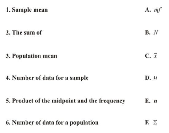
1. Match the words in the left column with the correct symbol from the right column.

The following table of grouped data represents the weights (in pounds) of all 100 babies born at a local hospital last year.

Weight (pounds)	Number of Babies
[3−5)	8
[5−7)	25
[7−9)	45
[9−11)	18
[11−13)	4

2. What is the summation of the values of mf for each class?
3. What is the value of N?
4. Calculate the mean weight for a baby.

The following table of grouped data represents the ages (in years) of 50 of the 500 teachers in a school district.

Age (years)	Number of Teachers
[25−35)	7
[35−45)	8
[45−55)	16
[55−65)	10
[65−75)	9

5. What is the summation of the values of mf for each class?
6. What is the value of n?
7. Calculate the mean age for a teacher.

The following table of grouped data represents the numbers of miles on all 25 cars in a used car lot.

Mileage	Number of Cars
[0−40,000)	3
[40,000−80,000)	6
[80,000−120,000)	10
[120,000−160,000)	4
[160,000−200,000)	2

8. What is the summation of the values of mf for each class?
9. What is the value of N?
10. Calculate the mean number of miles on a car.

---

Review (Answers)

To view the Review answers, open this PDF file and look for section 5.3.

---

Vocabulary

Term	Definition
grouped data	Grouped data is data that is placed in intervals.

---

Additional Resources

Video: Grouped Data to Find the Mean Principles

Activities: Grouped Data to Find the Mean Discussion Questions

Lesson Plans: Using Grouped Data to Find the Mean Lesson Plan

Practice: Grouped Data to Find the Mean

Real World: Grouped Data to Find the Mean 1