
9.8: Chi-Square Test
- Page ID
- 5790
\( \newcommand{\vecs}[1]{\overset { \scriptstyle \rightharpoonup} {\mathbf{#1}} } \)
\( \newcommand{\vecd}[1]{\overset{-\!-\!\rightharpoonup}{\vphantom{a}\smash {#1}}} \)
\( \newcommand{\dsum}{\displaystyle\sum\limits} \)
\( \newcommand{\dint}{\displaystyle\int\limits} \)
\( \newcommand{\dlim}{\displaystyle\lim\limits} \)
\( \newcommand{\id}{\mathrm{id}}\) \( \newcommand{\Span}{\mathrm{span}}\)
( \newcommand{\kernel}{\mathrm{null}\,}\) \( \newcommand{\range}{\mathrm{range}\,}\)
\( \newcommand{\RealPart}{\mathrm{Re}}\) \( \newcommand{\ImaginaryPart}{\mathrm{Im}}\)
\( \newcommand{\Argument}{\mathrm{Arg}}\) \( \newcommand{\norm}[1]{\| #1 \|}\)
\( \newcommand{\inner}[2]{\langle #1, #2 \rangle}\)
\( \newcommand{\Span}{\mathrm{span}}\)
\( \newcommand{\id}{\mathrm{id}}\)
\( \newcommand{\Span}{\mathrm{span}}\)
\( \newcommand{\kernel}{\mathrm{null}\,}\)
\( \newcommand{\range}{\mathrm{range}\,}\)
\( \newcommand{\RealPart}{\mathrm{Re}}\)
\( \newcommand{\ImaginaryPart}{\mathrm{Im}}\)
\( \newcommand{\Argument}{\mathrm{Arg}}\)
\( \newcommand{\norm}[1]{\| #1 \|}\)
\( \newcommand{\inner}[2]{\langle #1, #2 \rangle}\)
\( \newcommand{\Span}{\mathrm{span}}\) \( \newcommand{\AA}{\unicode[.8,0]{x212B}}\)
\( \newcommand{\vectorA}[1]{\vec{#1}} % arrow\)
\( \newcommand{\vectorAt}[1]{\vec{\text{#1}}} % arrow\)
\( \newcommand{\vectorB}[1]{\overset { \scriptstyle \rightharpoonup} {\mathbf{#1}} } \)
\( \newcommand{\vectorC}[1]{\textbf{#1}} \)
\( \newcommand{\vectorD}[1]{\overrightarrow{#1}} \)
\( \newcommand{\vectorDt}[1]{\overrightarrow{\text{#1}}} \)
\( \newcommand{\vectE}[1]{\overset{-\!-\!\rightharpoonup}{\vphantom{a}\smash{\mathbf {#1}}}} \)
\( \newcommand{\vecs}[1]{\overset { \scriptstyle \rightharpoonup} {\mathbf{#1}} } \)
\(\newcommand{\longvect}{\overrightarrow}\)
\( \newcommand{\vecd}[1]{\overset{-\!-\!\rightharpoonup}{\vphantom{a}\smash {#1}}} \)
\(\newcommand{\avec}{\mathbf a}\) \(\newcommand{\bvec}{\mathbf b}\) \(\newcommand{\cvec}{\mathbf c}\) \(\newcommand{\dvec}{\mathbf d}\) \(\newcommand{\dtil}{\widetilde{\mathbf d}}\) \(\newcommand{\evec}{\mathbf e}\) \(\newcommand{\fvec}{\mathbf f}\) \(\newcommand{\nvec}{\mathbf n}\) \(\newcommand{\pvec}{\mathbf p}\) \(\newcommand{\qvec}{\mathbf q}\) \(\newcommand{\svec}{\mathbf s}\) \(\newcommand{\tvec}{\mathbf t}\) \(\newcommand{\uvec}{\mathbf u}\) \(\newcommand{\vvec}{\mathbf v}\) \(\newcommand{\wvec}{\mathbf w}\) \(\newcommand{\xvec}{\mathbf x}\) \(\newcommand{\yvec}{\mathbf y}\) \(\newcommand{\zvec}{\mathbf z}\) \(\newcommand{\rvec}{\mathbf r}\) \(\newcommand{\mvec}{\mathbf m}\) \(\newcommand{\zerovec}{\mathbf 0}\) \(\newcommand{\onevec}{\mathbf 1}\) \(\newcommand{\real}{\mathbb R}\) \(\newcommand{\twovec}[2]{\left[\begin{array}{r}#1 \\ #2 \end{array}\right]}\) \(\newcommand{\ctwovec}[2]{\left[\begin{array}{c}#1 \\ #2 \end{array}\right]}\) \(\newcommand{\threevec}[3]{\left[\begin{array}{r}#1 \\ #2 \\ #3 \end{array}\right]}\) \(\newcommand{\cthreevec}[3]{\left[\begin{array}{c}#1 \\ #2 \\ #3 \end{array}\right]}\) \(\newcommand{\fourvec}[4]{\left[\begin{array}{r}#1 \\ #2 \\ #3 \\ #4 \end{array}\right]}\) \(\newcommand{\cfourvec}[4]{\left[\begin{array}{c}#1 \\ #2 \\ #3 \\ #4 \end{array}\right]}\) \(\newcommand{\fivevec}[5]{\left[\begin{array}{r}#1 \\ #2 \\ #3 \\ #4 \\ #5 \\ \end{array}\right]}\) \(\newcommand{\cfivevec}[5]{\left[\begin{array}{c}#1 \\ #2 \\ #3 \\ #4 \\ #5 \\ \end{array}\right]}\) \(\newcommand{\mattwo}[4]{\left[\begin{array}{rr}#1 \amp #2 \\ #3 \amp #4 \\ \end{array}\right]}\) \(\newcommand{\laspan}[1]{\text{Span}\{#1\}}\) \(\newcommand{\bcal}{\cal B}\) \(\newcommand{\ccal}{\cal C}\) \(\newcommand{\scal}{\cal S}\) \(\newcommand{\wcal}{\cal W}\) \(\newcommand{\ecal}{\cal E}\) \(\newcommand{\coords}[2]{\left\{#1\right\}_{#2}}\) \(\newcommand{\gray}[1]{\color{gray}{#1}}\) \(\newcommand{\lgray}[1]{\color{lightgray}{#1}}\) \(\newcommand{\rank}{\operatorname{rank}}\) \(\newcommand{\row}{\text{Row}}\) \(\newcommand{\col}{\text{Col}}\) \(\renewcommand{\row}{\text{Row}}\) \(\newcommand{\nul}{\text{Nul}}\) \(\newcommand{\var}{\text{Var}}\) \(\newcommand{\corr}{\text{corr}}\) \(\newcommand{\len}[1]{\left|#1\right|}\) \(\newcommand{\bbar}{\overline{\bvec}}\) \(\newcommand{\bhat}{\widehat{\bvec}}\) \(\newcommand{\bperp}{\bvec^\perp}\) \(\newcommand{\xhat}{\widehat{\xvec}}\) \(\newcommand{\vhat}{\widehat{\vvec}}\) \(\newcommand{\uhat}{\widehat{\uvec}}\) \(\newcommand{\what}{\widehat{\wvec}}\) \(\newcommand{\Sighat}{\widehat{\Sigma}}\) \(\newcommand{\lt}{<}\) \(\newcommand{\gt}{>}\) \(\newcommand{\amp}{&}\) \(\definecolor{fillinmathshade}{gray}{0.9}\)The Chi-Square Distribution
To analyze patterns between distinct categories, such as genders, political candidates, locations, or preferences, we use the chi-square goodness-of-fit test.
This test is used when estimating how closely a sample matches the expected distribution (also known as the goodness-of-fit test) and when estimating if two random variables are independent of one another (also known as the test of independence).
In this lesson, we will learn more about the goodness-of-fit test and how to create and evaluate hypotheses using this test.
The chi-square distribution can be used to perform the goodness-of-fit test, which compares the observed values of a categorical variable with the expected values of that same variable.
Constructing a Contingency Table
We would use the chi-square goodness-of-fit test to evaluate if there was a preference in the type of lunch that 11th grade students bought in the cafeteria. For this type of comparison, it helps to make a table to visualize the problem. We could construct the following table, known as a contingency table, to compare the observed and expected values.
Research Question: Do 11th grade students prefer a certain type of lunch?
Using a sample of 100 11th grade students, we recorded the following information:
| Type of Lunch | Observed Frequency | Expected Frequency |
|---|---|---|
| Salad | 21 | 25 |
| Sub Sandwich | 29 | 25 |
| Daily Special | 14 | 25 |
| Brought Own Lunch | 36 | 25 |
If there is no difference in which type of lunch is preferred, we would expect the students to prefer each type of lunch equally. To calculate the expected frequency of each category when assuming school lunch preferences are distributed equally, we divide the number of observations by the number of categories. Since there are 100 observations and 4 categories, the expected frequency of each category is 1004, or 25.
The Chi-Square Statistic
The value that indicates the comparison between the observed and expected frequency is called the chi-square statistic. The idea is that if the observed frequency is close to the expected frequency, then the chi-square statistic will be small. On the other hand, if there is a substantial difference between the two frequencies, then we would expect the chi-square statistic to be large.
To calculate the chi-square statistic, χ2, we use the following formula:
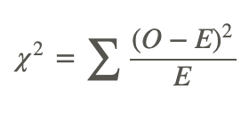
where:
χ2 is the chi-square test statistic.
O is the observed frequency value for each event.
E is the expected frequency value for each event.
We compare the value of the test statistic to a tabled chi-square value to determine the probability that a sample fits an expected pattern.
Features of the Goodness-of-Fit Test
As mentioned, the goodness-of-fit test is used to determine patterns of distinct categorical variables. The test requires that the data are obtained through a random sample. The number of degrees of freedom associated with a particular chi-square test is equal to the number of categories minus one. That is, df=c−1.
Using our example about the preferences for types of school lunches, we calculate the degrees of freedom as follows:
df3=number of categories−1=4−1
There are many situations that use the goodness-of-fit test, including surveys, taste tests, and analysis of behaviors. Interestingly, goodness-of-fit tests are also used in casinos to determine if there is cheating in games of chance, such as cards or dice. For example, if a certain card or number on a die shows up more than expected (a high observed frequency compared to the expected frequency), officials use the goodness-of-fit test to determine the likelihood that the player may be cheating or that the game may not be fair.
Testing Hypotheses
Let’s use our original example to create and test a hypothesis using the goodness-of-fit chi-square test. First, we will need to state the null and alternative hypotheses for our research question. Since our research question asks, “Do 11th grade students prefer a certain type of lunch?” our null hypothesis for the chi-square test would state that there is no difference between the observed and the expected frequencies. Therefore, our alternative hypothesis would state that there is a significant difference between the observed and expected frequencies.
Null Hypothesis
H0:O=E (There is no statistically significant difference between observed and expected frequencies.)
Alternative Hypothesis
Ha:O≠E (There is a statistically significant difference between observed and expected frequencies.)
Also, the number of degrees of freedom for this test is 3.
Using an alpha level of 0.05, we look under the column for 0.05 and the row for degrees of freedom, which, again, is 3. According to the standard chi-square distribution table, we see that the critical value for chi-square is 7.815. Therefore, we would reject the null hypothesis if the chi-square statistic is greater than 7.815.
Note that we can calculate the chi-square statistic with relative ease.
| Type of Lunch | Observed Frequency | Expected Frequency | (O−E)2/E |
|---|---|---|---|
| Salad | 21 | 25 | 0.64 |
| Sub Sandwich | 29 | 25 | 0.64 |
| Daily Special | 14 | 25 | 4.84 |
| Brought Own Lunch | 36 | 25 | 4.84 |
| Total (chi-square) | 10.96 |
Since our chi-square statistic of 10.96 is greater than 7.815, we reject the null hypotheses and accept the alternative hypothesis. Therefore, we can conclude that there is a significant difference between the types of lunches that 11th grade students prefer.
Using the Chi-Square Goodness of Fit Test
A game involves rolling 3 dice. The winnings are directly proportional to the number of fives rolled. Suppose someone plays the game 100 times with the following observed counts:
| Number of Fives | Observed Number of rolls |
|---|---|
| 0 | 48 |
| 1 | 35 |
| 2 | 15 |
| 3 | 2 |
Someone becomes suspicious and wants to determine whether the dice are fair.
If the dice are fair the probability of rolling a 5 is 1/6. If we roll 3 dice, independently then the number fives in three rolls is distributed as a Binomial (3,1/6).
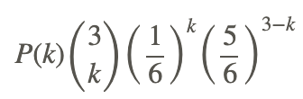
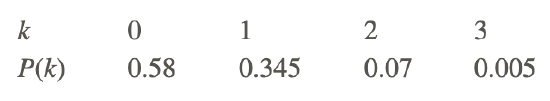
a. Determine the probability of 0, 1, 2 and 3 fives under this distribution.
Since we have a binomial distribution with 3 independent trials and probability of success 1/6 on each trial, we can compute the probabilities using either the TI Calculator binompdf(3,1/6, k) where k represents the particular value in which we are interested or we can use the formula
b. Determine if the dice are fair (Use a chi-square goodness of fit test).
First you must find the expected number of rolls for each category. To do this, multiply the probability of each category by 100. For example, the expected number of rolls where you observe zero 5's is 0.5787⋅100=57.87. The formula for the chi-square goodness of fit test is 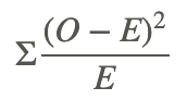
where O represents the observed and E represents the expected. You can do this calculation on the TI Calculator by putting the observed values in List 1, the Expected values in List 2, and in List 3 put  .
.
| Number of Fives | Observed Number of rolls | Expected Number of rolls | (O−E)2E |
|---|---|---|---|
| 0 | 48 | 58 | 1.72 |
| 1 | 35 | 34.5 | 0.007 |
| 2 | 15 | 7 | 9.14 |
| 3 | 2 | 0.5 | 4.5 |
You then sum the values in List 3. This will be the value of your chi-square statistic:
χ2=1.72+0.007+9.14+4.5=15.367
In the previous example, we saw that the critical value for a chi-squared statistic at the 0.05 level of significance is 7.815. Since χ2=15.367>7.815, at the .05 level of significance, we can reject the null hypothesis and conclude that the dice are not fair.
Example
Example 1
The marital status distribution of the U.S. Female population, age 18 and older, is as shown below.
| Marital Status | Proportion |
|---|---|
| Never married | 0.227 |
| Married | 0.557 |
| Widowed | 0.98 |
| Divorced/separated | 0.117 |
(Source: US Census Bureau, “America’s Families and Living Arrangements, 2008)
Suppose a random sample of 400 US young adult females, 18-24 years old, yielded the following frequency distribution. Does this age group of females fit the distribution of the US adult population?
| Marital Status | Frequency |
|---|---|
| Never married | 238 |
| Married | 140 |
| Widowed | 3 |
| Divorced/separated | 19 |
In this problem you determine the expect number for each category by multiplying the proportion by 400, the total number of people in the study.
| Marital Status | Observed | Expected | (O−E)2/E |
|---|---|---|---|
| Divorced/separated | 19 | 46.8 | 16.51 |
| Married | 140 | 222.8 | 30.77 |
| Widowed | 3 | 39.2 | 33.43 |
| Never married | 238 | 90.8 | 238.63 |
The chi-square statistic is 238.63 + 30.77 + 33.43 + 16.51 = 319.34 with 3 degrees of freedom. The p-value is 0.00. The decision, at the 0.05 and 0.01 levels of significance, is to reject the null hypothesis. With a goodness-of-fit test, the null hypothesis is always that the two data sets have the same distribution. Since we are rejecting the null hypothesis, this means that this age group of young adult females does not fit the distribution of the US adult population.
Review
- What is the name of the statistical test used to analyze the patterns between two categorical variables?
- Student’s t-test
- the ANOVA test
- the chi-square test
- the z-score
- There are two types of chi-square tests. Which type of chi-square test estimates how closely a sample matches an expected distribution?
- the goodness-of-fit test
- the test for independence
- Which of the following is considered a categorical variable?
- income
- gender
- height
- weight
- If there were 250 observations in a data set and 2 uniformly distributed categories that were being measured, the expected frequency for each category would be:
- 125
- 500
- 250
- 5
- What is the formula for calculating the chi-square statistic?
- A principal is planning a field trip. She samples a group of 100 students to see if they prefer a sporting event, a play at the local college, or a science museum. She records the following results:
| Type of Field Trip | Number Preferring |
|---|---|
| Sporting Event | 53 |
| Play | 18 |
| Science Museum | 29 |
(a) What is the observed frequency value for the Science Museum category?
(b) What is the expected frequency value for the Sporting Event category?
(c) What would be the null hypothesis for the situation above?
(i) There is no preference between the types of field trips that students prefer.
(ii) There is a preference between the types of field trips that students prefer.
(d) What would be the chi-square statistic for the research question above?
(e) If the estimated chi-square level of significance was 5.99, would you reject or fail to reject the null hypothesis?
- In 1982 in Western Australia, 1317 males and 854 females died of heart disease, 1119 males and 828 females died of cancer, 371 males and 460 females died of cerebral vascular disease and 346 males and 147 females died of accidents. (source: www.statsci.org/data/z/deathwa.html) Put this information into a contingency table.
- For each of the following situations, give the p-value for the given chi-square statistic.
- χ2=3.84,df=1
- χ2=6.7 for a table with 3 rows and 3 columns
- χ2=26.23 for a table with 2 rows and 3 columns
- Determine the critical value in each of the following situations.
- Level of significance is 05, degrees of freedom = 1
- Level of significance is 0.01; table has 3 rows and 4 columns
- Level of significance is 0.05, degrees of freedom = 8
- For each of the following situations determine if the result is statistically significant at the 0.5 level.
- χ2=2.89,df=1
- χ2=23.60,df=4
- Are the situations in problem 10 statistically significant at the .01 level?
- In the following situations, give the expected count for each of the k categories:
- k=3,H0:p1=p2=p3=1/3,n=300
- k=3,H0:p1=1/4,p2=1/4,p3=1/2,n=1000
- Explain whether each of these is possible in a chi-square goodness of fit test.
- The chi-square statistic is negative.
- The chi-square statistic is 0.
- A 6-sided die is rolled 120 times. Conduct a hypothesis test to determine if the die is fair. The data below are the result of the 120 rolls.
| Face Value | Frequency |
|---|---|
| 1 | 29 |
| 2 | 15 |
| 3 | 15 |
| 4 | 16 |
| 5 | 15 |
| 6 | 30 |
- True or False: (if false rewrite so it is true). As the degrees of freedom increase, the graph of the chi-square distribution looks more and more symmetrical.
- True or False: (if false rewrite so it is true). In a goodness of fit test the expected values are the values we would expect if the null hypothesis were true.
- True or False: (if false rewrite so it is true). Use a goodness of fit test to determine if high school principals believe that students are absent equally during the week or not.
- True or False: (if false rewrite so it is true). For a chi-square distribution with 17 degrees of freedom, the probability that a value is greater than 20 is 0.7248.
- Suppose an investigator conducts a study of the relationship between gender (male or female) and book preference (fiction or nonfiction) of children 12 years old.
- Suppose the p-value of the study is not small enough to reject the null hypothesis. Write this conclusion in the context of the situation.
- Now suppose the p-value of the study is small enough to reject the null hypothesis. In the context of the situation, express the conclusion in two different ways.
- Suppose a car dealer offers cars in three different colors: silver, black and white. In a sample of 111 buyers, 59 chose black, 25 chose silver and the remainder chose white. Is there sufficient evidence to conclude that the colors are not equally preferred? Carry out a significance test and be sure to state the null hypothesis and the population to which your conclusion applies.
- The manufacturer of M&Ms states, on the website, the color distribution of M&Ms. Access the website to discover the claim of the manufacturer. Purchase and combine a number of 1-lb bags of M&Ms. Are the observed results statistically significant from the claim of the manufacturer.
Vocabulary
| Term | Definition |
|---|---|
| chi-squared distribution | The distribution of the chi-square statistic is called the chi-square distribution. |
| chi-squared goodness of fit test | The chi-square goodness of fit test can be used to estimate how closely an observed distribution matches an expected distribution. |
| chi-squared statistic | The chi-squared statistic (X^2) is used to evaluate how well a set of observed data fits a corresponding expected set. |
| chi-squared test | The chi-squared test calculates the probability that a given distribution is a good fit for observed data. |
| contingency tables | A contingency table (two-way table) is used to organize data from multiple categories of two variables so that various assessments may be made. |
| degrees of freedom | Degrees of freedom are essentially the number of samples that have the ‘freedom’ to change without necessarily affecting the sample mean. Degrees of freedom has the formula df = n - 1. |
| test for independence | The test for independence is used when estimating if two random variables are independent of one another. |
| test of significance | A test of significance (calculating a z-score or a t-statistic) is done when a claim is made about the value of a population parameter. |
Additional Resources
Video: Example of a Goodness-of-Fit Test
Practice: Chi-Square Test