11.2: Biosignatures
- Page ID
- 5642
\( \newcommand{\vecs}[1]{\overset { \scriptstyle \rightharpoonup} {\mathbf{#1}} } \)
\( \newcommand{\vecd}[1]{\overset{-\!-\!\rightharpoonup}{\vphantom{a}\smash {#1}}} \)
\( \newcommand{\id}{\mathrm{id}}\) \( \newcommand{\Span}{\mathrm{span}}\)
( \newcommand{\kernel}{\mathrm{null}\,}\) \( \newcommand{\range}{\mathrm{range}\,}\)
\( \newcommand{\RealPart}{\mathrm{Re}}\) \( \newcommand{\ImaginaryPart}{\mathrm{Im}}\)
\( \newcommand{\Argument}{\mathrm{Arg}}\) \( \newcommand{\norm}[1]{\| #1 \|}\)
\( \newcommand{\inner}[2]{\langle #1, #2 \rangle}\)
\( \newcommand{\Span}{\mathrm{span}}\)
\( \newcommand{\id}{\mathrm{id}}\)
\( \newcommand{\Span}{\mathrm{span}}\)
\( \newcommand{\kernel}{\mathrm{null}\,}\)
\( \newcommand{\range}{\mathrm{range}\,}\)
\( \newcommand{\RealPart}{\mathrm{Re}}\)
\( \newcommand{\ImaginaryPart}{\mathrm{Im}}\)
\( \newcommand{\Argument}{\mathrm{Arg}}\)
\( \newcommand{\norm}[1]{\| #1 \|}\)
\( \newcommand{\inner}[2]{\langle #1, #2 \rangle}\)
\( \newcommand{\Span}{\mathrm{span}}\) \( \newcommand{\AA}{\unicode[.8,0]{x212B}}\)
\( \newcommand{\vectorA}[1]{\vec{#1}} % arrow\)
\( \newcommand{\vectorAt}[1]{\vec{\text{#1}}} % arrow\)
\( \newcommand{\vectorB}[1]{\overset { \scriptstyle \rightharpoonup} {\mathbf{#1}} } \)
\( \newcommand{\vectorC}[1]{\textbf{#1}} \)
\( \newcommand{\vectorD}[1]{\overrightarrow{#1}} \)
\( \newcommand{\vectorDt}[1]{\overrightarrow{\text{#1}}} \)
\( \newcommand{\vectE}[1]{\overset{-\!-\!\rightharpoonup}{\vphantom{a}\smash{\mathbf {#1}}}} \)
\( \newcommand{\vecs}[1]{\overset { \scriptstyle \rightharpoonup} {\mathbf{#1}} } \)
\( \newcommand{\vecd}[1]{\overset{-\!-\!\rightharpoonup}{\vphantom{a}\smash {#1}}} \)
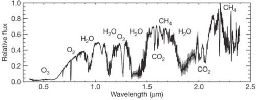
\(\newcommand{\avec}{\mathbf a}\) \(\newcommand{\bvec}{\mathbf b}\) \(\newcommand{\cvec}{\mathbf c}\) \(\newcommand{\dvec}{\mathbf d}\) \(\newcommand{\dtil}{\widetilde{\mathbf d}}\) \(\newcommand{\evec}{\mathbf e}\) \(\newcommand{\fvec}{\mathbf f}\) \(\newcommand{\nvec}{\mathbf n}\) \(\newcommand{\pvec}{\mathbf p}\) \(\newcommand{\qvec}{\mathbf q}\) \(\newcommand{\svec}{\mathbf s}\) \(\newcommand{\tvec}{\mathbf t}\) \(\newcommand{\uvec}{\mathbf u}\) \(\newcommand{\vvec}{\mathbf v}\) \(\newcommand{\wvec}{\mathbf w}\) \(\newcommand{\xvec}{\mathbf x}\) \(\newcommand{\yvec}{\mathbf y}\) \(\newcommand{\zvec}{\mathbf z}\) \(\newcommand{\rvec}{\mathbf r}\) \(\newcommand{\mvec}{\mathbf m}\) \(\newcommand{\zerovec}{\mathbf 0}\) \(\newcommand{\onevec}{\mathbf 1}\) \(\newcommand{\real}{\mathbb R}\) \(\newcommand{\twovec}[2]{\left[\begin{array}{r}#1 \\ #2 \end{array}\right]}\) \(\newcommand{\ctwovec}[2]{\left[\begin{array}{c}#1 \\ #2 \end{array}\right]}\) \(\newcommand{\threevec}[3]{\left[\begin{array}{r}#1 \\ #2 \\ #3 \end{array}\right]}\) \(\newcommand{\cthreevec}[3]{\left[\begin{array}{c}#1 \\ #2 \\ #3 \end{array}\right]}\) \(\newcommand{\fourvec}[4]{\left[\begin{array}{r}#1 \\ #2 \\ #3 \\ #4 \end{array}\right]}\) \(\newcommand{\cfourvec}[4]{\left[\begin{array}{c}#1 \\ #2 \\ #3 \\ #4 \end{array}\right]}\) \(\newcommand{\fivevec}[5]{\left[\begin{array}{r}#1 \\ #2 \\ #3 \\ #4 \\ #5 \\ \end{array}\right]}\) \(\newcommand{\cfivevec}[5]{\left[\begin{array}{c}#1 \\ #2 \\ #3 \\ #4 \\ #5 \\ \end{array}\right]}\) \(\newcommand{\mattwo}[4]{\left[\begin{array}{rr}#1 \amp #2 \\ #3 \amp #4 \\ \end{array}\right]}\) \(\newcommand{\laspan}[1]{\text{Span}\{#1\}}\) \(\newcommand{\bcal}{\cal B}\) \(\newcommand{\ccal}{\cal C}\) \(\newcommand{\scal}{\cal S}\) \(\newcommand{\wcal}{\cal W}\) \(\newcommand{\ecal}{\cal E}\) \(\newcommand{\coords}[2]{\left\{#1\right\}_{#2}}\) \(\newcommand{\gray}[1]{\color{gray}{#1}}\) \(\newcommand{\lgray}[1]{\color{lightgray}{#1}}\) \(\newcommand{\rank}{\operatorname{rank}}\) \(\newcommand{\row}{\text{Row}}\) \(\newcommand{\col}{\text{Col}}\) \(\renewcommand{\row}{\text{Row}}\) \(\newcommand{\nul}{\text{Nul}}\) \(\newcommand{\var}{\text{Var}}\) \(\newcommand{\corr}{\text{corr}}\) \(\newcommand{\len}[1]{\left|#1\right|}\) \(\newcommand{\bbar}{\overline{\bvec}}\) \(\newcommand{\bhat}{\widehat{\bvec}}\) \(\newcommand{\bperp}{\bvec^\perp}\) \(\newcommand{\xhat}{\widehat{\xvec}}\) \(\newcommand{\vhat}{\widehat{\vvec}}\) \(\newcommand{\uhat}{\widehat{\uvec}}\) \(\newcommand{\what}{\widehat{\wvec}}\) \(\newcommand{\Sighat}{\widehat{\Sigma}}\) \(\newcommand{\lt}{<}\) \(\newcommand{\gt}{>}\) \(\newcommand{\amp}{&}\) \(\definecolor{fillinmathshade}{gray}{0.9}\)One important method for searching for life on other worlds is to search for the by-products of life that contaminate planetary atmospheres. Oxygen alone or methane alone would not be good biosignatures, but the combination of oxygen and methane is a smoking gun for life. At the temperatures and pressures in the atmosphere of Earth, oxygen would react quickly with methane, producing carbon dioxide and water. The simultaneous existence of these elements on Earth only occurs because life is producing these elements and maintaining chemical disequilibrium.
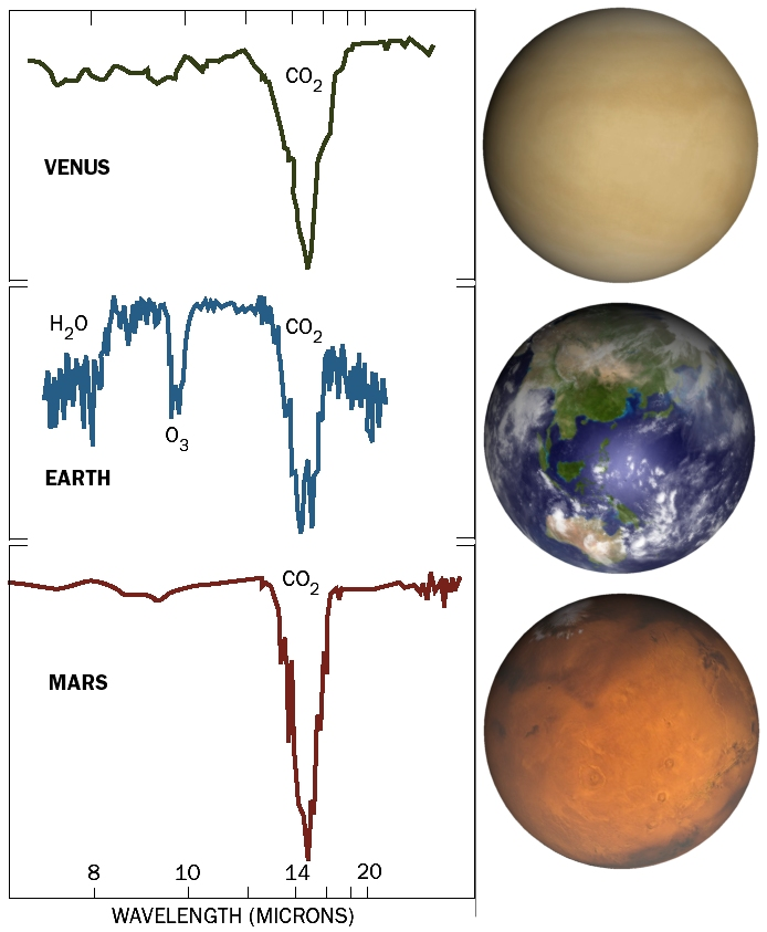
The Figure below compares a spectrum of the atmosphere of Venus, Earth and Mars. The Earth spectrum contains a biosignature: oxygen and methane (not labeled). The presence of water also suggests that Earth is a habitable world. In contrast, atmospheric spectra of Venus and Mars do not have these same indicators for life.
Atmosphere Spectroscopy
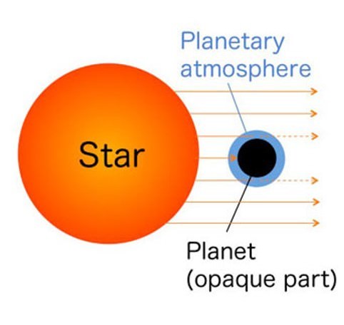
When a planet transits, some of the light from the star penetrates the atmosphere of the planet where atoms and molecules will absorb light from the star. This gives us a spectrum of the (star + planet). When the planet is eclipsed by the star, another observation will produce a spectrum of the star-only. We can divide the (star + planet) spectrum by the (star-only) spectrum to obtain a spectrum of the planet atmosphere.
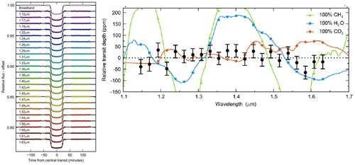
The planetary spectrum is usually quite faint so a good strategy is to photometrically observe the transit with several different filters. This technique is called spectrophotometry and gives very low resolution information about the planetary atmosphere. Then, the planetary spectrum can be compared to synthetic models with different chemical compositions. A poor match is rejected and a good match is retained as a plausible solution. The figure below (left) shows an example of transit observations taken through different filters. Each of those measurements is a measure of intensity at a particular wavelength that is plotted on the right (filled black circles with error bars for the uncertainty in the flux). The observed spectrum on the right has overplotted models: 100% methane (green), 100% water (blue) and 100% carbon dioxide (orange). The first two models can be rejected and the last model can be retained. Further observations and additional synthetic models can be used to identify or rule out other possible atmospheric spectra.
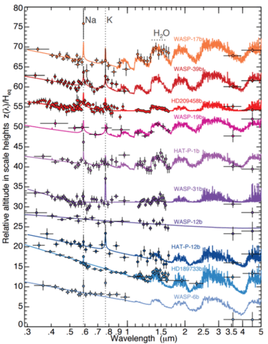
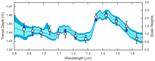
The figure below shows the likely detection of a water feature in the atmosphere of Wasp-12b, a hot Jupiter. The next figure shows spectra from a survey of hot Jupiters using the Hubble Space Telescope. The James Webb Space Telescope (JWST) will be launched in 2021 and will try to determine the compositions of atmospheres of rocky planets around M dwarfs.
Question for Thought
Recall that the transit depth is determined by the ratio of the planetary ratio to the stellar radius squared, \(\left(\frac{R_{planet}}{R_{star}}\right)^2\). With this in mind, why are hot Jupiters particularly conducive to transit spectroscopy for solar type stars? What is the advantage offered by M dwarfs?
The Red Edge
Another spectral feature that might be a good indicator of life is the appearance of a red edge in spectra. On Earth, the red edge is a property of chlorophyll, which becomes abruptly reflective at infrared wavelengths.
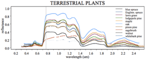
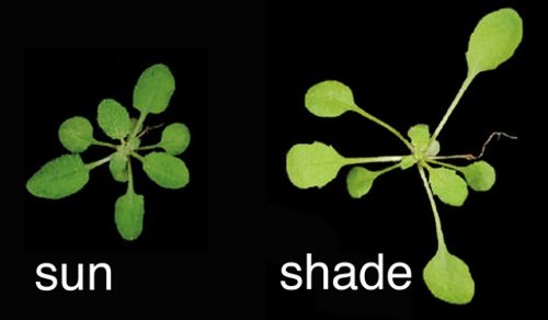
This property of chlorophyll keeps plants from overheating, but is also integral to plants growing efficiently through a process called shade avoidance. Plants are capable of detecting a lack of infrared light and this triggers a response in plants that produces longer stems and larger leaves, which allows a plant to capture more sunlight.
Photosynthetic organisms were a critical step in the evolution of aerobic respiration in eukaryotes. Therefore, a similar detection in the atmospheres of other planets would be an intriguing clue for bio-activity. The red edge is a strong signal in the atmospheric spectra from Earth and an easy feature to search for in the atmospheres of other planets.