
7.3: The Doppler Technique
- Page ID
- 5636
\( \newcommand{\vecs}[1]{\overset { \scriptstyle \rightharpoonup} {\mathbf{#1}} } \)
\( \newcommand{\vecd}[1]{\overset{-\!-\!\rightharpoonup}{\vphantom{a}\smash {#1}}} \)
\( \newcommand{\dsum}{\displaystyle\sum\limits} \)
\( \newcommand{\dint}{\displaystyle\int\limits} \)
\( \newcommand{\dlim}{\displaystyle\lim\limits} \)
\( \newcommand{\id}{\mathrm{id}}\) \( \newcommand{\Span}{\mathrm{span}}\)
( \newcommand{\kernel}{\mathrm{null}\,}\) \( \newcommand{\range}{\mathrm{range}\,}\)
\( \newcommand{\RealPart}{\mathrm{Re}}\) \( \newcommand{\ImaginaryPart}{\mathrm{Im}}\)
\( \newcommand{\Argument}{\mathrm{Arg}}\) \( \newcommand{\norm}[1]{\| #1 \|}\)
\( \newcommand{\inner}[2]{\langle #1, #2 \rangle}\)
\( \newcommand{\Span}{\mathrm{span}}\)
\( \newcommand{\id}{\mathrm{id}}\)
\( \newcommand{\Span}{\mathrm{span}}\)
\( \newcommand{\kernel}{\mathrm{null}\,}\)
\( \newcommand{\range}{\mathrm{range}\,}\)
\( \newcommand{\RealPart}{\mathrm{Re}}\)
\( \newcommand{\ImaginaryPart}{\mathrm{Im}}\)
\( \newcommand{\Argument}{\mathrm{Arg}}\)
\( \newcommand{\norm}[1]{\| #1 \|}\)
\( \newcommand{\inner}[2]{\langle #1, #2 \rangle}\)
\( \newcommand{\Span}{\mathrm{span}}\) \( \newcommand{\AA}{\unicode[.8,0]{x212B}}\)
\( \newcommand{\vectorA}[1]{\vec{#1}} % arrow\)
\( \newcommand{\vectorAt}[1]{\vec{\text{#1}}} % arrow\)
\( \newcommand{\vectorB}[1]{\overset { \scriptstyle \rightharpoonup} {\mathbf{#1}} } \)
\( \newcommand{\vectorC}[1]{\textbf{#1}} \)
\( \newcommand{\vectorD}[1]{\overrightarrow{#1}} \)
\( \newcommand{\vectorDt}[1]{\overrightarrow{\text{#1}}} \)
\( \newcommand{\vectE}[1]{\overset{-\!-\!\rightharpoonup}{\vphantom{a}\smash{\mathbf {#1}}}} \)
\( \newcommand{\vecs}[1]{\overset { \scriptstyle \rightharpoonup} {\mathbf{#1}} } \)
\(\newcommand{\longvect}{\overrightarrow}\)
\( \newcommand{\vecd}[1]{\overset{-\!-\!\rightharpoonup}{\vphantom{a}\smash {#1}}} \)
\(\newcommand{\avec}{\mathbf a}\) \(\newcommand{\bvec}{\mathbf b}\) \(\newcommand{\cvec}{\mathbf c}\) \(\newcommand{\dvec}{\mathbf d}\) \(\newcommand{\dtil}{\widetilde{\mathbf d}}\) \(\newcommand{\evec}{\mathbf e}\) \(\newcommand{\fvec}{\mathbf f}\) \(\newcommand{\nvec}{\mathbf n}\) \(\newcommand{\pvec}{\mathbf p}\) \(\newcommand{\qvec}{\mathbf q}\) \(\newcommand{\svec}{\mathbf s}\) \(\newcommand{\tvec}{\mathbf t}\) \(\newcommand{\uvec}{\mathbf u}\) \(\newcommand{\vvec}{\mathbf v}\) \(\newcommand{\wvec}{\mathbf w}\) \(\newcommand{\xvec}{\mathbf x}\) \(\newcommand{\yvec}{\mathbf y}\) \(\newcommand{\zvec}{\mathbf z}\) \(\newcommand{\rvec}{\mathbf r}\) \(\newcommand{\mvec}{\mathbf m}\) \(\newcommand{\zerovec}{\mathbf 0}\) \(\newcommand{\onevec}{\mathbf 1}\) \(\newcommand{\real}{\mathbb R}\) \(\newcommand{\twovec}[2]{\left[\begin{array}{r}#1 \\ #2 \end{array}\right]}\) \(\newcommand{\ctwovec}[2]{\left[\begin{array}{c}#1 \\ #2 \end{array}\right]}\) \(\newcommand{\threevec}[3]{\left[\begin{array}{r}#1 \\ #2 \\ #3 \end{array}\right]}\) \(\newcommand{\cthreevec}[3]{\left[\begin{array}{c}#1 \\ #2 \\ #3 \end{array}\right]}\) \(\newcommand{\fourvec}[4]{\left[\begin{array}{r}#1 \\ #2 \\ #3 \\ #4 \end{array}\right]}\) \(\newcommand{\cfourvec}[4]{\left[\begin{array}{c}#1 \\ #2 \\ #3 \\ #4 \end{array}\right]}\) \(\newcommand{\fivevec}[5]{\left[\begin{array}{r}#1 \\ #2 \\ #3 \\ #4 \\ #5 \\ \end{array}\right]}\) \(\newcommand{\cfivevec}[5]{\left[\begin{array}{c}#1 \\ #2 \\ #3 \\ #4 \\ #5 \\ \end{array}\right]}\) \(\newcommand{\mattwo}[4]{\left[\begin{array}{rr}#1 \amp #2 \\ #3 \amp #4 \\ \end{array}\right]}\) \(\newcommand{\laspan}[1]{\text{Span}\{#1\}}\) \(\newcommand{\bcal}{\cal B}\) \(\newcommand{\ccal}{\cal C}\) \(\newcommand{\scal}{\cal S}\) \(\newcommand{\wcal}{\cal W}\) \(\newcommand{\ecal}{\cal E}\) \(\newcommand{\coords}[2]{\left\{#1\right\}_{#2}}\) \(\newcommand{\gray}[1]{\color{gray}{#1}}\) \(\newcommand{\lgray}[1]{\color{lightgray}{#1}}\) \(\newcommand{\rank}{\operatorname{rank}}\) \(\newcommand{\row}{\text{Row}}\) \(\newcommand{\col}{\text{Col}}\) \(\renewcommand{\row}{\text{Row}}\) \(\newcommand{\nul}{\text{Nul}}\) \(\newcommand{\var}{\text{Var}}\) \(\newcommand{\corr}{\text{corr}}\) \(\newcommand{\len}[1]{\left|#1\right|}\) \(\newcommand{\bbar}{\overline{\bvec}}\) \(\newcommand{\bhat}{\widehat{\bvec}}\) \(\newcommand{\bperp}{\bvec^\perp}\) \(\newcommand{\xhat}{\widehat{\xvec}}\) \(\newcommand{\vhat}{\widehat{\vvec}}\) \(\newcommand{\uhat}{\widehat{\uvec}}\) \(\newcommand{\what}{\widehat{\wvec}}\) \(\newcommand{\Sighat}{\widehat{\Sigma}}\) \(\newcommand{\lt}{<}\) \(\newcommand{\gt}{>}\) \(\newcommand{\amp}{&}\) \(\definecolor{fillinmathshade}{gray}{0.9}\)Indirect detection
The Doppler technique (also called the radial velocity technique) was the first method to successfully detect exoplanets orbiting sun-like stars. This technique measures the velocity of stars over time. The "radial" part of "radial velocity" comes from the fact that only the component of the velocity along our line of site ("radial") can be measured using the Doppler effect.
All stars are traveling in orbits around the center of our Milky Way galaxy. For example, the Sun takes about 220 Myr to complete one loop around the galaxy. As the Sun travels around the galaxy, some stars appear to be moving toward us while others are moving away.
After subtracting the constant galactic velocity for a given star, a residual small periodic wobble in the velocity of a star can reveal that the star is being tugged around a common center of mass by another body, as shown in the figure below. These residual velocities can be modeled to determine whether the orbiting object is a planet. With the Doppler technique, the planet is never observed (making this an "indirect" detection method). Instead, the time-varying velocity of the host star is modeled to infer the presence of an unseen planet.
To recap: all stars have some nearly constant radial velocity; stars that exhibit a residual periodicity in their radial velocities have a gravitationally bound companion.
How do you measure the velocity of a star?
The Doppler technique makes use of the fact that light is a wave and as the source of light (the star) is moving toward us or away from us, the frequency of the light emitted by the star is blue-shifted or red-shifted (by the "Doppler effect"). Doppler shifts are measured from the spectrum of a star, where the stellar flux (the photons of light from the star that are captured by the detector) is sorted into component wavelengths.
The figure below shows an "echelle'' spectrum where the rainbow spectrum of light has been cleverly chopped and stacked by the optics of the instrument (a spectrograph). The spectrum spans the entire visible wavelength range from 400 - 700 nm and each row of the spectrum spans roughly 10 nm. In this spectrum, there are thousands of dark spectral absorption lines corresponding to wavelengths where specific atomic transitions occur (e.g., hydrogen, sodium iron and magnesium absorption lines are identified below) and absorb emerging light in the atmosphere of the star.

After recording the echelle spectrum with a low noise digital camera, the image is transformed into a more manageable format by extracting each row or order into a series of arrays (an example of this array near the two sodium lines in the echelle image above is shown in the figure above). Each pixel in the array (sometimes called a 1-d spectrum) contains the stellar flux and the calibrated wavelength of the light.
The absorption features in a stellar spectrum reveal the composition of the star, but they can also be used to measure the radial velocity of the star. The velocity of the star, \(v\), can be calculated from the non-relativistic Doppler equation by measuring the wavelength shift for each of the absorption lines:
\[\frac{\Delta\lambda}{\lambda}\,=\frac{v}{c}\]
where \(\Delta\lambda\) is the average shift measured for thousands of absorption lines,
\(\lambda\) is the known rest wavelength of each absorption line,
\(c\) is the speed of light (299,792,458 m/s).
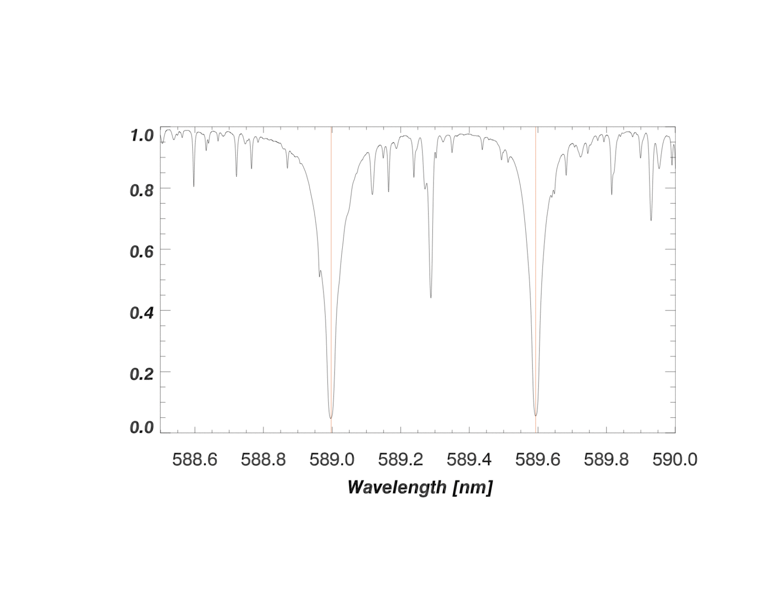
A segment of the 1-d extracted spectrum around the deep pair of sodium absorption lines is shown in the image below. A decrease in flux (i.e., and absorption line) occurs wherever there is an atomic transition that absorbs light from the star. In the animation below, each shift of the spectrum simulates a different velocity shift. By measuring the periodic shift of the wavelengths for these lines (\(\Delta\lambda\)) relative to the rest wavelength (\(\lambda\), indicated by the red vertical lines for sodium), the velocity of the star over time can be calculated.
The animation above is an extreme exaggeration (for the purpose of illustration) of the reflex Doppler shift that would occur from orbiting exoplanets. The spectral absorption lines in the animation above are between 5 - 20 pixels in width. A spectral line shift of just one pixel on a detector corresponds to a radial velocity change of about 1000 m/s. The amplitude of Doppler shifts caused by exoplanets would be invisible to the eye on the scale shown above.
Our ability to detect smaller planets is limited by the precision with which we can measure the shifts of spectral lines. Jupiter induces a radial velocity in the sun of about 12 m/s with a periodicity of about 12 years. To detect Jupiter, we would need to measure a 12-year back-and-forth shift in the spectral lines of 0.01 pixel. This requires that we control the stability of our instrument to much better than this precision and maintain the control over at least 12 years. Impressively, this is the state of the art - astronomers can measure wavelength shifts to the level of 0.001 pixel (1 m/s) with decades-long stability. However, detecting the stellar reflex velocity from a planet like the Earth is a much greater challenge. The Earth induces a velocity of about 10 cm/s in the Sun. This corresponds to a one-year back and forth shift of 0.0001 pixel. New instruments are now being developed to try to find other examples of Earth-like planets that might harbor life.
Detecting planets from velocities
To detect a planet with the Doppler technique, many spectra must be obtained that span the complete orbital period of the star-planet system. Of course, astronomers don't know the orbital period in advance, so in practice, they take as many spectra as possible and then use mathematical and statistical methods to search for repeating changes in the radial velocity.
The figure below depicts the orbit of a star as a dashed circular path that is viewed edge-on by an observer to the right. The velocity of the star is constant in this figure, however the projected radial velocity along our line of site is changing. At point A, the star moves toward the observer and the spectrum of the star is blue-shifted (the measured wavelengths are shorter). At point E, the star moves away from the observer and the spectrum of the star is red-shifted (the measured wavelengths are shifted to longer, redder wavelengths). At point C, there is no radial velocity - all of the motion is tangential to our line of site. At points B and D, only the projected radial component of the velocity (velocity times the sine of the orbital inclination) can be measured in the stellar spectrum.

The orbit of the planet cannot be seen; instead we model the time series radial velocity measurements of the star to infer several attributes of the orbit:
- the velocity amplitude, \(K\)
- the orbital period, \(P\)
- orbital eccentricity, \(e\)
- rotation of the orbit, \(\omega\)
- time of periastron passage, \(T_p\)
These parameters can then be used to calculate the semi-major axis and the mass of the planet times the orbital inclination using Newtonian physics.
\[K\,=\frac{8.95[cm/s]}{\sqrt{1-e^2}}\,\frac{m_{pl}\sin i}{m_{\oplus}}\,\left(\frac{M_{\ast} + m_{pl}}{M_{\odot}}\right)^{-2/3}\left(\frac{P}{year}\right)^{-1/3}\]
- where \(K\) is the velocity semi-amplitude in cm/s,
- \(m_{pl}\sin i\) is the mass of the planet in units of Earth masses times the sine of the orbital inclination,
- \(m_{\oplus}\) is the mass of the Earth - so the ratio \(\frac{m_{pl}}{m_{\oplus}}\) is dimensionless,
- \(M_{\ast}\) is the mass of the star - the mass of the planet can be considered negligible and dropped,
- \(M_{\odot}\) is the mass of the sun, so the ratio \(\frac{M_{\ast}}{M_{\odot}}\) is dimensionless,
- \(P\) is the orbital period in years (so this ratio is also dimensionless).
Conceptual Questions
What is the value of \(K\) if \(m_{pl}\sin i\,=\,1m\_{\oplus},\,M_{\ast} \,=\,1M_{\odot},\,e=0\,\text{and}\,P=1\,year\)?
Qualitatively, how does the value of K change if the orbital eccentricity is greater than zero?
Qualitatively, how does the value of change if the orbital period is less than one year?
Why mpl sin i?
Equation 2 relates the radial velocity amplitude of the star to \(m_{pl}\sin i\), rather than to the actual mass of the planet. What does that mean? The Doppler technique measures the projected 1-dimensional velocities of stars. When an orbit is viewed edge-on (\(\sin i\)=90∘) we see the full amplitude of this sinusoidally varying projection. If an orbit is face-on (\(\sin i\)=0∘) there is no radial component to the stellar velocity; the orbit is undetectable with this technique. For orbits that are inclined in between these values, the velocity semi-amplitude, \(K\), decreases with the sine of the inclination. We cannot distinguish whether \(K\) is smaller because the orbiting mass or the inclination is smaller; we only model the product \(m_{pl}\sin i\). The true mass is given by:
\[m_{pl}\,=\,\frac{m_{pl}\sin i}{\sin i}\]
While we cannot solve for inclination, equation 3 shows that because \(\sin i\) ranges between 0 and 1, \(m_{pl}\sin i\) is a lower limit to the true mass of the planet.
Statistical probability for sin i
For randomly oriented inclinations, the probability of drawing a particular \(\sin i\) is not uniform. Instead, the probability of observing an orbit with an inclination \(\Delta i\) between \(i_1\) and \(i_2\) scales as the difference between the cosine of those angles:
\[\mathcal{P}\,=\,|\cos i_1\,-\cos i_2|\]
So, there is an 86% probability that the inclination of a random orbit is between 90∘ and 30∘. For these typical orbits, the true mass of the planet would be within a factor of two of the measured \(m_{pl}\sin i\). Conversely, there is only a 14% probability that an orbital inclination is between 30∘ and 0∘ (yielding a true mass more than twice \(m_{pl}\sin i\)).
Real world examples
In 1995, Michel Mayor and Didier Queloz discovered the first exoplanet around a main sequence star using the Doppler technique. The planet that they discovered has a mass similar to Jupiter, and orbits the star 51 Pegasi once every 4.23 days. The data from their 1995 discovery paper are shown in the figure below. Because the signal repeats, the velocities can be folded so that the orbital periods repeat. This "phase-folded" data is a helpful way to display relatively short periodic signals and clearly demonstrates that the signal is repeating in a predictable way.
In the data from the Mayor & Queloz 1995 paper, you can see that from September to November in 1994, the radial velocities for 51 Pegasi were changing. This perplexed Didier Queloz, who was a graduate student working with Professor Mayor. To better understand the velocity variations, he began taking more data. Mayor and Queloz developed a mathematical model (shown as the solid line) that fits the velocity changes of the star and also describes Keplerian orbital motion. It is quite an empowering feeling to develop a model like this and to then watch the future velocities of the star follow your predictions.

Queloz and Mayor could not quite believe what they were seeing. A Jupiter-mass planet in a 4-day orbit was very different than any of the planets in our solar system. In their paper, they discuss the alternative interpretations such as stellar pulsations and effectively rule them out. They conclude that the most likely interpretation is an orbiting planetary mass companion.
Because they derive \(m_{planet}\sin i\), they note that the true mass may be larger than one Jupiter mass. Some skeptics believed that Mayor and Queloz had simply detected a stellar binary system that was oriented nearly face-on. However, an inclination of less than 1∘ is required to pump \(m_{pl}\sin i\) up to the stellar mass regime of 70 Jupiter masses. According to equation 4, there is only 1 chance in 10,000 that they would have observed such a low inclination orbit.
The next few exoplanets
Mayor and Queloz's discovery of an exoplanet in such a short orbital period was a game-changer. A team of astronomers at San Francisco State University, Marcy and Butler, were also trying to find exoplanets using the Doppler technique. They had a backlog of data because they were collecting about 50 spectra per night, but it took 24 hours to analyze a single spectra on the slower computers of the day. Spurred on by the discovery of 51 Peg b, Sun Microsystems made a donation to the SFSU team and they quickly crunched through their observations, discovering Jupiter like planets around 70 Virginis and 47 Ursa Majoris in their sample of 120 stars. The second of these, 47 UMa b, was very much like 51 Peg b - a Jupiter mass planet in an orbit of just a few days.
However, the data for 70 Vir b (shown below) told a different story.

Instead of the sinusoidal velocity variation seen with 51 Peg b, this planet has a more peaked velocity variation revealing an orbit with eccentricity of 0.4. The planet mass (6.6 times the mass of Jupiter) is also much larger, producing greater velocity variations in 70 Virginis. To the skeptics, the discovery of yet another massive planet was further support of the idea that nearly face-on binary star systems were being discovered rather than exoplanets. The fact that this object was in an eccentric orbit added to the doubts - planets in our solar system are in nearly circular orbits. Surely the rest of the cosmos would be like us?
Practice with the radial velocity simulator
There are a lot of concepts to understand with the Doppler technique. First, we use the spectrum of the star to measure wavelength shifts that correspond to changes in the velocity of the star. Second, we only see the projected radial component of the stellar velocity (this leads to a sinusoidal variation in the signal). Third, we don't know the inclination of the orbit - this tilt of the orbit means that the sinusoidal signal will be largest when viewed edge-on (90∘ inclination) and smaller as the inclination tilts toward face-on. This means that we only measure \(m_{planet}\sin i\) with the Doppler method.
Let's walk through a series of exercises with the Nebraska Astronomy Applet Project (NAAP) simulator to help develop your intuition and understanding of the Doppler method. You will need to download the Simulations package (will install in your Applications directory, open Extrasolar Planets, Exoplanet Radial Velocity Simulator).
Begin by opening the simulator and setting up the inputs to match the values shown in the figure below. Simulated radial velocities are "phase-folded'' in the upper right hand plot. The radial velocities are obtained as a function of time, but if you repeat observations over more than one orbital period, the data can be folded so that all of the peaks and troughs of the curve line up. This is routinely done by astronomers to build evidence for repeating signals.

Simulation Exercises
- First, make sure that you understand what the orbit visualizations are showing in the upper left corner of the control panel. There are four different views:
- side view - looking edge-on at the orbit
- earth view - the orbit is now tilted by the 76.8 degrees that you specified.
- orbit view - this is looking at the orbit face-on
- 3-d view with arrows indicating viewing angles for 1 and 2 above.
- Now, rotate the inclination bar and notice two things: the tilt of the orbit changes in the earth view panel and the amplitude of the RV signal decreases as the inclination goes toward zero and increases as the inclination goes to 90∘.
- Reset the inclination to 76.8∘. Now increase the number of observations from 30 to 300 to see how confidence increases with more data.
- Toggle the "theoretical curve" off and slide the "noise" bar (representing the measurement precision) from 1 m/s to 12 m/s. When the measurement uncertainty (noise) is comparable to the signal (12 m/s) it is only possible to have a convincing detection if there are many observations. As you dial down the number of observations from 300 back to 30, the underlying signal is less certain.
- Check to see how the mass of the star affects the amplitude of the RV signal (notice that the numbers on the y-axis will change). A lower mass star is easier for a planet to push around than a high mass star.
- The Earth has a mass that is 0.0032 times the mass of Jupiter. Change the mass in the simulator to this value. Is there any way of convincingly detecting an Earth analog (Earth mass planet at 1 AU) around a solar mass star with the precision of the simulator? Are there any orbits where you could convincingly detect an Earth mass planet (i.e., any mass star, any semi-major axis)?