1.2.2: Discrete and Continuous Functions

Continuity and Discontinuity

Continuity is a property of functions that can be drawn without lifting your pencil. Some functions, like the reciprocal functions, have two distinct parts that are unconnected. Functions that are unconnected are discontinuous. What are the three ways functions can be discontinuous and how do they come about?

---

Continuity and Discontinuity of Functions

Functions that can be drawn without lifting up your pencil are called continuous functions. You will define continuous in a more mathematically rigorous way after you study limits.

There are three types of discontinuities: Removable, Jump and Infinite.

Removable Discontinuities

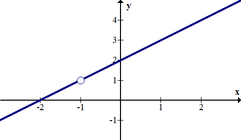
Removable discontinuities occur when a rational function has a factor with an x that exists in both the numerator and the denominator. Removable discontinuities are shown in a graph by a hollow circle that is also known as a hole. Below is the graph for \(\ f(x)=\frac{(x+2)(x+1)}{x+1}\). Notice that it looks just like y=x+2 except for the hole at x=−1. When graphing function, you should cancel the removable factor, graph like usual and then insert a hole in the appropriate spot at the end. There is a hole at x=−1 because when \(\ x=-1, f(x)=\frac{0}{0}\)

[Figure1]

Removable discontinuities can be “filled in” if you make the function a piecewise function and define a part of the function at the point where the hole is. In the example above, to make f(x) continuous you could redefine it as:

\(\ f(x)=\left\{\begin{array}{ll}
\frac{(x+2)(x+1)}{x+1}, & x \neq-1 \\
1, & x=-1
\end{array}\right.\)

Jump Discontinuities

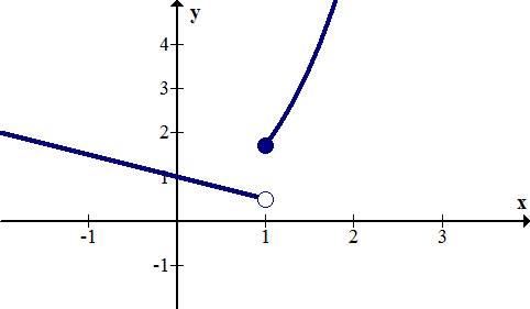
Jump discontinuities occur when a function has two ends that don’t meet even if the hole is filled in. In order to satisfy the vertical line test and make sure the graph is truly that of a function, only one of the end points may be filled. Below is an example of a function with a jump discontinuity.

[Figure2]

Infinite Discontinuities

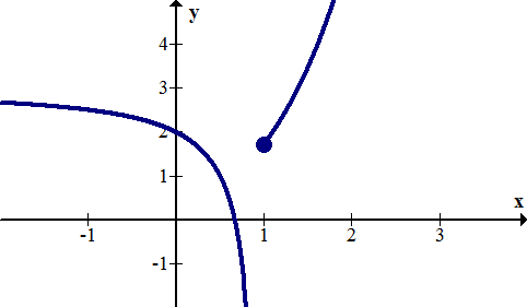
Infinite discontinuities occur when a function has a vertical asymptote on one or both sides. This is shown in the graph of the function below at x=1.

[Figure3]

---

Examples

Example 1

Solution

Earlier you were asked how functions can be discontinuous. There are three ways that functions can be discontinuous. When a rational function has a vertical asymptote as a result of the denominator being equal to zero at some point, it will have an infinite discontinuity at that point. When the numerator and denominator of a rational function have one or more of the same factors, there will be removable discontinuities corresponding to each of these factors. Finally, when the different parts of a piecewise function don’t “match”, there will be a jump discontinuity.

Example 2

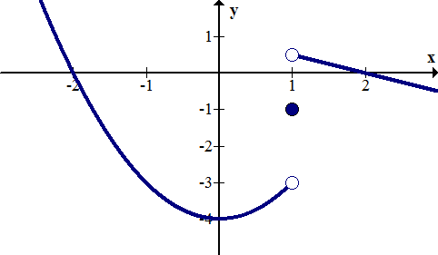
Identify the discontinuity of the piecewise function graphically.

\(\ f(x)=\left\{\begin{array}{ll}
x^{2}-4 & x<1 \\
-1 & x=1 \\
-\frac{1}{2} x+1 & x>1
\end{array}\right.\)

[Figure4]

Solution

There is a jump discontinuity at x=1. The piecewise function describes a function in three parts; a parabola on the left, a single point in the middle and a line on the right.

Example 3

Describe the continuity or discontinuity of the function \(\ f(x)=\sin \left(\frac{1}{x}\right)\)

[Figure5]

Solution

The function seems to oscillate infinitely as x approaches zero. One thing that the graph fails to show is that 0 is clearly not in the domain. The graph does not shoot to infinity, nor does it have a simple hole or jump discontinuity. Calculus and Real Analysis are required to state more precisely what is going on.

Example 4

Describe the discontinuities of the function below.

[Figure6]

Solution

There is a jump discontinuity at x=−1 and an infinite discontinuity at x=2.

Example 5

Describe the discontinuities of the function below.

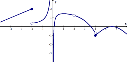[Figure7]

Solution

There are jump discontinuities at x=−2 and x=4. There is a removable discontinuity at x=2. There is an infinite discontinuity at x=0.

---

Review

Describe any discontinuities in the functions below:

1. y=x

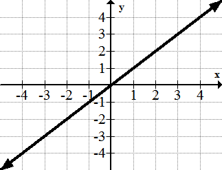[Figure8]

2. y=x²

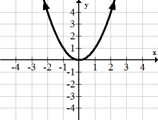[Figure9]

3. y=x³

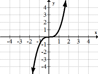[Figure10]

4. \(\ y=\sqrt{x}\)

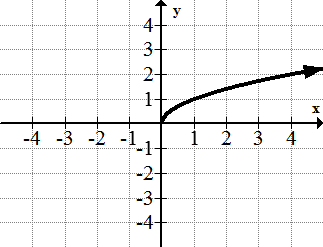[Figure11]

5. \(\ y=\frac{1}{x}\)

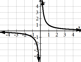[Figure12]

6. y=e^x

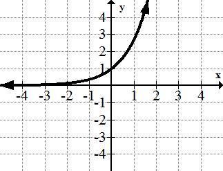[Figure13]

7. y=ln(x)

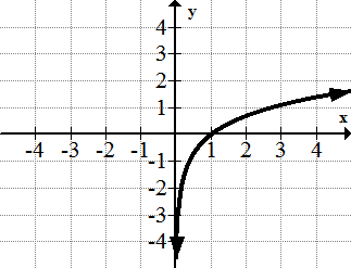[Figure14]

8. \(\ y=\frac{1}{1+e^{-x}}\)

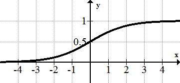[Figure15]

9.

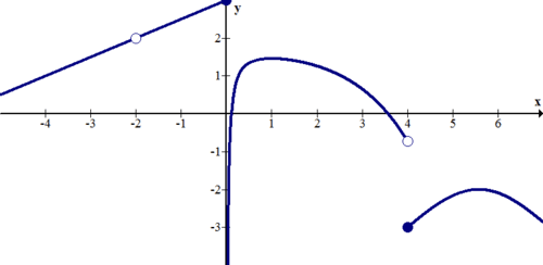[Figure16]

10.

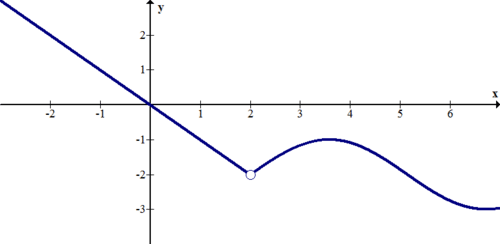[Figure17]

11.

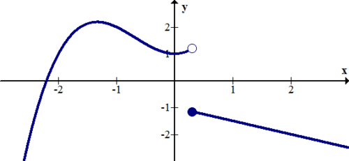[Figure18]

12. f(x) has a jump discontinuity at x=3, a removable discontinuity at x=5, and another jump discontinuity at x=6. Draw a picture of a graph that could be f(x).

13. g(x) has a jump discontinuity at x=−2, an infinite discontinuity at x=1, and another jump discontinuity at x=3. Draw a picture of a graph that could be g(x).

14. h(x) has a removable discontinuity at x=−4, a jump discontinuity at x=1, and another jump discontinuity at x=7. Draw a picture of a graph that could be h(x).

15. j(x) has an infinite discontinuity at x=0, a removable discontinuity at x=1, and a jump discontinuity at x=4. Draw a picture of a graph that could be j(x).

---

Review (Answers)

To see the Review answers, open this PDF file and look for section 1.10.

---

Vocabulary

Term	Definition
Continuous	Continuity for a point exists when the left and right sided limits match the function evaluated at that point. For a function to be continuous, the function must be continuous at every single point in an unbroken domain.
discontinuities	The points of discontinuity for a function are the input values of the function where the function is discontinuous.
Discrete	A relation is said to be discrete if there are a finite number of data points on its graph. Graphs of discrete relations appear as dots.
Function	A function is a relation where there is only one output for every input. In other words, for every value of x, there is only one value for y.
Infinite discontinuities	Infinite discontinuities occur when a function has a vertical asymptote on one or both sides. This will happen when a factor in the denominator of the function is zero.
Infinite discontinuity	Infinite discontinuities occur when a function has a vertical asymptote on one or both sides. This will happen when a factor in the denominator of the function is zero.
interval	An interval is a specific and limited part of a function.
Jump discontinuities	Inverse functions are functions that 'undo' each other. Formally f(x) and g(x) are inverse functions if f(g(x))=g(f(x))=x.
Removable discontinuities	Removable discontinuities are also known as holes. They occur when factors can be algebraically canceled from rational functions.
Removable discontinuity	Removable discontinuities are also known as holes. They occur when factors can be algebraically canceled from rational functions.

---

Image Attributions

1. [Figure 1]
   Credit: CK-12 Foundation
   License: CC BY-SA
2. [Figure 2]
   Credit: CK-12 Foundation
   Source: https://www.flickr.com/photos/jhaymesisvip/6497720753/
   License: CC BY-SA
3. [Figure 3]
   Credit: CK-12 Foundation
   License: CC BY-SA
4. [Figure 4]
   Credit: CK-12 Foundation
   License: CC BY-SA
5. [Figure 5]
   Credit: CK-12 Foundation
   License: CC BY-SA
6. [Figure 6]
   Credit: CK-12 Foundation
   Source: https://www.flickr.com/photos/jhaymesisvip/6497720753/
   License: CC BY-SA
7. [Figure 7]
   Credit: CK-12 Foundation
   License: CC BY-SA
8. [Figure 8]
   Credit: CK-12 Foundation
   License: CC BY-SA
9. [Figure 9]
   Credit: CK-12 Foundation
   License: CC BY-SA
10. [Figure 10]
    Credit: CK-12 Foundation
    Source: http://classconnection.s3.amazonaws.com/753/flashcards/449753/png/screen_shot_2011-09-21_at_8.07.32_pm1316650094429.png
    License: CC BY-SA
11. [Figure 11]
    Credit: CK-12 Foundation
    License: CC BY-SA
12. [Figure 12]
    Credit: CK-12 Foundation
    License: CC BY-SA
13. [Figure 13]
    Credit: CK-12 Foundation
    License: CC BY-SA
14. [Figure 14]
    Credit: CK-12 Foundation
    License: CC BY-SA
15. [Figure 15]
    Credit: CK-12 Foundation;Paula Evans;Rob Young
    Source: https://www.flickr.com/photos/rob-young/1149735229/;https://commons.wikimedia.org/wiki/File:Will_%26_Grace_Apartment_Building_(1149735229).jpg
    License: CC BY-SA; CC BY-NC-SA
16. [Figure 16]
    Credit: CK-12 Foundation
    License: CC BY-SA
17. [Figure 17]
    Credit: CK-12 Foundation
    License: CC BY-SA
18. [Figure 18]
    Credit: CK-12 Foundation
    License: CC BY-SA