1.4.3: Graphing Cube Root Functions
- Page ID
- 14137
\( \newcommand{\vecs}[1]{\overset { \scriptstyle \rightharpoonup} {\mathbf{#1}} } \)
\( \newcommand{\vecd}[1]{\overset{-\!-\!\rightharpoonup}{\vphantom{a}\smash {#1}}} \)
\( \newcommand{\dsum}{\displaystyle\sum\limits} \)
\( \newcommand{\dint}{\displaystyle\int\limits} \)
\( \newcommand{\dlim}{\displaystyle\lim\limits} \)
\( \newcommand{\id}{\mathrm{id}}\) \( \newcommand{\Span}{\mathrm{span}}\)
( \newcommand{\kernel}{\mathrm{null}\,}\) \( \newcommand{\range}{\mathrm{range}\,}\)
\( \newcommand{\RealPart}{\mathrm{Re}}\) \( \newcommand{\ImaginaryPart}{\mathrm{Im}}\)
\( \newcommand{\Argument}{\mathrm{Arg}}\) \( \newcommand{\norm}[1]{\| #1 \|}\)
\( \newcommand{\inner}[2]{\langle #1, #2 \rangle}\)
\( \newcommand{\Span}{\mathrm{span}}\)
\( \newcommand{\id}{\mathrm{id}}\)
\( \newcommand{\Span}{\mathrm{span}}\)
\( \newcommand{\kernel}{\mathrm{null}\,}\)
\( \newcommand{\range}{\mathrm{range}\,}\)
\( \newcommand{\RealPart}{\mathrm{Re}}\)
\( \newcommand{\ImaginaryPart}{\mathrm{Im}}\)
\( \newcommand{\Argument}{\mathrm{Arg}}\)
\( \newcommand{\norm}[1]{\| #1 \|}\)
\( \newcommand{\inner}[2]{\langle #1, #2 \rangle}\)
\( \newcommand{\Span}{\mathrm{span}}\) \( \newcommand{\AA}{\unicode[.8,0]{x212B}}\)
\( \newcommand{\vectorA}[1]{\vec{#1}} % arrow\)
\( \newcommand{\vectorAt}[1]{\vec{\text{#1}}} % arrow\)
\( \newcommand{\vectorB}[1]{\overset { \scriptstyle \rightharpoonup} {\mathbf{#1}} } \)
\( \newcommand{\vectorC}[1]{\textbf{#1}} \)
\( \newcommand{\vectorD}[1]{\overrightarrow{#1}} \)
\( \newcommand{\vectorDt}[1]{\overrightarrow{\text{#1}}} \)
\( \newcommand{\vectE}[1]{\overset{-\!-\!\rightharpoonup}{\vphantom{a}\smash{\mathbf {#1}}}} \)
\( \newcommand{\vecs}[1]{\overset { \scriptstyle \rightharpoonup} {\mathbf{#1}} } \)
\(\newcommand{\longvect}{\overrightarrow}\)
\( \newcommand{\vecd}[1]{\overset{-\!-\!\rightharpoonup}{\vphantom{a}\smash {#1}}} \)
\(\newcommand{\avec}{\mathbf a}\) \(\newcommand{\bvec}{\mathbf b}\) \(\newcommand{\cvec}{\mathbf c}\) \(\newcommand{\dvec}{\mathbf d}\) \(\newcommand{\dtil}{\widetilde{\mathbf d}}\) \(\newcommand{\evec}{\mathbf e}\) \(\newcommand{\fvec}{\mathbf f}\) \(\newcommand{\nvec}{\mathbf n}\) \(\newcommand{\pvec}{\mathbf p}\) \(\newcommand{\qvec}{\mathbf q}\) \(\newcommand{\svec}{\mathbf s}\) \(\newcommand{\tvec}{\mathbf t}\) \(\newcommand{\uvec}{\mathbf u}\) \(\newcommand{\vvec}{\mathbf v}\) \(\newcommand{\wvec}{\mathbf w}\) \(\newcommand{\xvec}{\mathbf x}\) \(\newcommand{\yvec}{\mathbf y}\) \(\newcommand{\zvec}{\mathbf z}\) \(\newcommand{\rvec}{\mathbf r}\) \(\newcommand{\mvec}{\mathbf m}\) \(\newcommand{\zerovec}{\mathbf 0}\) \(\newcommand{\onevec}{\mathbf 1}\) \(\newcommand{\real}{\mathbb R}\) \(\newcommand{\twovec}[2]{\left[\begin{array}{r}#1 \\ #2 \end{array}\right]}\) \(\newcommand{\ctwovec}[2]{\left[\begin{array}{c}#1 \\ #2 \end{array}\right]}\) \(\newcommand{\threevec}[3]{\left[\begin{array}{r}#1 \\ #2 \\ #3 \end{array}\right]}\) \(\newcommand{\cthreevec}[3]{\left[\begin{array}{c}#1 \\ #2 \\ #3 \end{array}\right]}\) \(\newcommand{\fourvec}[4]{\left[\begin{array}{r}#1 \\ #2 \\ #3 \\ #4 \end{array}\right]}\) \(\newcommand{\cfourvec}[4]{\left[\begin{array}{c}#1 \\ #2 \\ #3 \\ #4 \end{array}\right]}\) \(\newcommand{\fivevec}[5]{\left[\begin{array}{r}#1 \\ #2 \\ #3 \\ #4 \\ #5 \\ \end{array}\right]}\) \(\newcommand{\cfivevec}[5]{\left[\begin{array}{c}#1 \\ #2 \\ #3 \\ #4 \\ #5 \\ \end{array}\right]}\) \(\newcommand{\mattwo}[4]{\left[\begin{array}{rr}#1 \amp #2 \\ #3 \amp #4 \\ \end{array}\right]}\) \(\newcommand{\laspan}[1]{\text{Span}\{#1\}}\) \(\newcommand{\bcal}{\cal B}\) \(\newcommand{\ccal}{\cal C}\) \(\newcommand{\scal}{\cal S}\) \(\newcommand{\wcal}{\cal W}\) \(\newcommand{\ecal}{\cal E}\) \(\newcommand{\coords}[2]{\left\{#1\right\}_{#2}}\) \(\newcommand{\gray}[1]{\color{gray}{#1}}\) \(\newcommand{\lgray}[1]{\color{lightgray}{#1}}\) \(\newcommand{\rank}{\operatorname{rank}}\) \(\newcommand{\row}{\text{Row}}\) \(\newcommand{\col}{\text{Col}}\) \(\renewcommand{\row}{\text{Row}}\) \(\newcommand{\nul}{\text{Nul}}\) \(\newcommand{\var}{\text{Var}}\) \(\newcommand{\corr}{\text{corr}}\) \(\newcommand{\len}[1]{\left|#1\right|}\) \(\newcommand{\bbar}{\overline{\bvec}}\) \(\newcommand{\bhat}{\widehat{\bvec}}\) \(\newcommand{\bperp}{\bvec^\perp}\) \(\newcommand{\xhat}{\widehat{\xvec}}\) \(\newcommand{\vhat}{\widehat{\vvec}}\) \(\newcommand{\uhat}{\widehat{\uvec}}\) \(\newcommand{\what}{\widehat{\wvec}}\) \(\newcommand{\Sighat}{\widehat{\Sigma}}\) \(\newcommand{\lt}{<}\) \(\newcommand{\gt}{>}\) \(\newcommand{\amp}{&}\) \(\definecolor{fillinmathshade}{gray}{0.9}\)Graphing Cubed Root Functions
Mrs. Garcia assigns her student the cube root function \(\ y=-\sqrt[3]{(x+1)}\) to graph for homework. The following day, she asks her students which quadrant(s) their graph is in.
Alendro says that because of the negative sign, all y values are negative. Therefore his graph is only in the third and fourth quadrants quadrant.
Dako says that his graph is in the third and fourth quadrants as well but it is also in the second quadrant.
Marisha says they are both wrong and that her graph of the function is in all four quadrants.
Which one of them is correct?
Graphing Cubed Root Functions
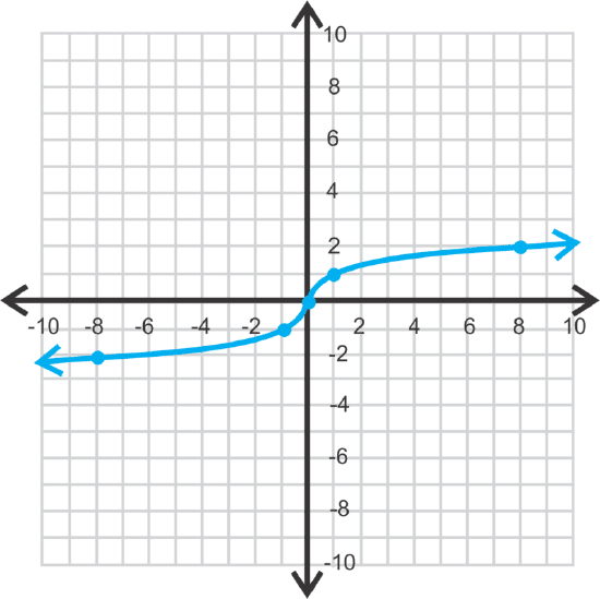
A cubed root function is different from that of a square root. Their general forms look very similar, \(\ y=a \sqrt[3]{x-h}+k\) and the parent graph is \(\ y=\sqrt[3]{x}\). However, we can take the cubed root of a negative number, therefore, it will be defined for all values of x. Graphing the parent graph, we have:
 [Figure1]
| x | y |
|---|---|
| -27 | -3 |
| -8 | -2 |
| -1 | -1 |
| 0 | 0 |
| 1 | 1 |
| 8 | 2 |
| 27 | 3 |
For \(\ y=\sqrt[3]{x}\), the output is the same as the input of \(\ y=x^{3}\). The domain and range of \(\ y=\sqrt[3]{x}\) are all real numbers. Notice there is no “starting point” like the square root functions, the (h,k) now refers to the point where the function bends, called a point of inflection.
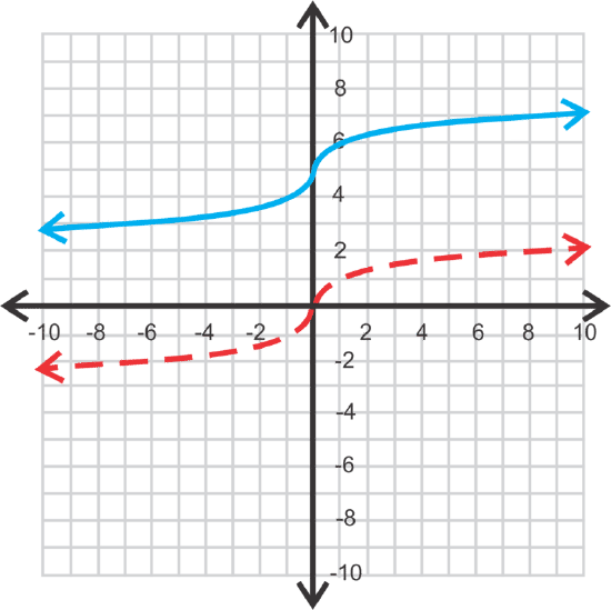
Let's describe how to obtain the graph of \(\ y=\sqrt[3]{x}+5\) from \(\ y=\sqrt[3]{x}\).
 [Figure2]
We know that the +5 indicates a vertical shift of 5 units up. Therefore, this graph will look exactly the same as the parent graph, shifted up five units.
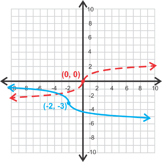
Now, let's graph \(\ f(x)=-\sqrt[3]{x+2}-3\) and find the domain and range.
 [Figure3]
From the previous problem, we know that from the parent graph, this function is going to shift to the left two units and down three units. The negative sign will result in a reflection.
Alternate Method: If you want to use a table, that will also work. Here is a table, then plot the points. (h,k) should always be the middle point in your table.
| x | y |
|---|---|
| 6 | -5 |
| -1 | -4 |
| -2 | -3 |
| -3 | -2 |
| -10 | -1 |
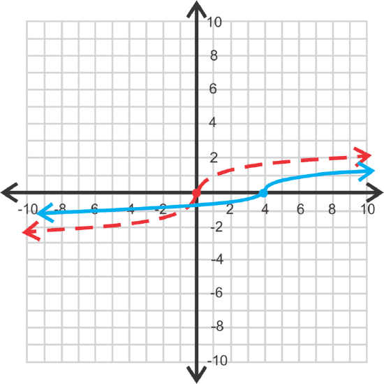
Finally, let's graph \(\ f(x)=\frac{1}{2} \sqrt[3]{x-4}\).
The -4 tells us that, from the parent graph, the function will shift to the right four units. The \(\ 1 \over 2\) effects how quickly the function will “grow”. Because it is less than one, it will grow slower than the parent graph.
Using the graphing calculator: If you wanted to graph this function using the TI-83 or 84, press Y= and clear out any functions. Then, press (1÷2), MATH and scroll down to 4: \sqrt[3]{ } and press ENTER. Then, type in the rest of the function, so that \(\ Y=\left(\frac{1}{2}\right) \sqrt[3]{(X-4)}\). Press GRAPH and adjust the window.
Important Note: The domain and range of all cubed root functions are both all real numbers.
Solution
Earlier, you were asked to determine which student was correct.
If you graph the function \(\ y=-\sqrt[3]{(x+1)}\), you see that the domain is all real numbers, which makes all quadrants possible. However, for all positive values of x, y is negative because of the negative sign in front of the cube root. That rules out the first quadrant. Therefore, Dako is correct.
Evaluate \(\ y=\sqrt[3]{x+4}-11\) when \(\ x=−12\).
Solution
Plug in \(\ x=−12\) and solve for \(\ y\).
\(\ y=\sqrt[3]{-12+4}-11=\sqrt[3]{-8}+4=-2+4=2\)
Describe how to obtain the graph of \(\ y=\sqrt[3]{x+4}-11\) from \(\ y=\sqrt[3]{x}\).
Solution
Starting with \(\ y=\sqrt[3]{x}\), you would obtain \(\ y=\sqrt[3]{x+4}-11\) by shifting the function to the left four units and down 11 units.
Graph the following cubed root functions. Check your graphs on the graphing calculator.
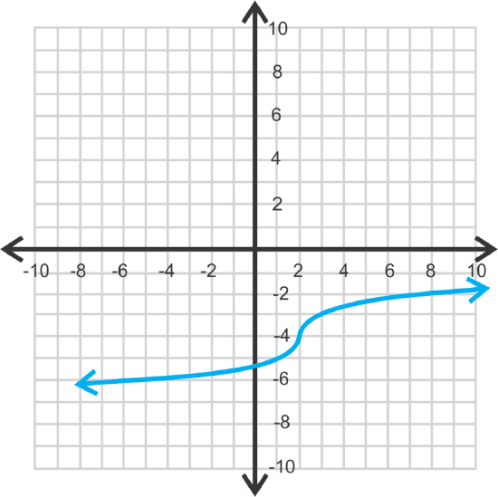
\(\ y=\sqrt[3]{x-2}-4\)
Solution
This function is a horizontal shift to the right two units and down four units.
 [Figure4]
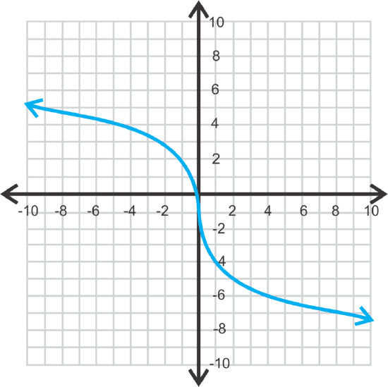
\(\ f(x)=-3 \sqrt{x}-1\)
Solution
This function is a reflection of \(\ y=\sqrt[3]{x}\) and stretched to be three times as large. Lastly, it is shifted down one unit.
 [Figure5]
Review
Evaluate \(\ f(x)=\sqrt[3]{2 x-1}\) for the following values of \(\ x\).
- f(14)
- f(−62)
- f(20)
Graph the following cubed root functions. Use your calculator to check your answers.
- \(\ y=\sqrt[3]{x}+4\)
- \(\ y=\sqrt[3]{x-3}\)
- \(\ f(x)=\sqrt[3]{x+2}-1\)
- \(\ g(x)=-\sqrt[3]{x}-6\)
- \(\ f(x)=2 \sqrt[3]{x+1}\)
- \(\ h(x)=-3 \sqrt[3]{x}+5\)
- \(\ y=\frac{1}{2} \sqrt[3]{1-x}\)
- \(\ y=2 \sqrt[3]{x+4}-3\)
- \(\ y=-\frac{1}{3} \sqrt[3]{x-5}+2\)
- \(\ g(x)=\sqrt[3]{6-x}+7\)
- \(\ f(x)=-5 \sqrt[3]{x-1}+3\)
- \(\ y=4 \sqrt[3]{7-x}-8\)
Vocabulary
| Term | Definition |
|---|---|
| General Equation for a Cubed Root Function | The general equation for a cubed root function is \(\ f(x)=a \sqrt[3]{x-h}+k\), where h is the horizontal shift and k is the vertical shift. |
Image Attributions
- [Figure 1]
Credit: Sean MacEntee
Source: https://www.flickr.com/photos/smemon/17323618152/in/photolist-soQ58A-5rouLK-67pQ1V-a54ocN-51ysYT-pP1VGr-6gshc-d8RVdu-nBXVi8-Nv9px-qtm3yn-dUUJmL-6ojCxV-DejJUS-51yqZg-51yqk4-5NrFcF-51CE4o-51CD2w-51CEao-51yqf8-fdo2Jf-51ypZi-51CDos-F9SKny-51CEmJ-jnS68-51ysyc-4t1z5J-51yqat-51CCQU-d9VTUC-51ypzB-2hVbrU-29Gjnh-4Q2TH4-ayVtXQ-6ooPqQ-51CEA9-agFDN7-51ypHi-51CGdY-51CFMG-51ysUK-anJz1-51yrta-51yuA8-51CFPY-51ysrz-51CFG1 - [Figure 2]
Credit: Sean MacEntee
Source: https://www.flickr.com/photos/smemon/17323618152/in/photolist-soQ58A-5rouLK-67pQ1V-a54ocN-51ysYT-pP1VGr-6gshc-d8RVdu-nBXVi8-Nv9px-qtm3yn-dUUJmL-6ojCxV-DejJUS-51yqZg-51yqk4-5NrFcF-51CE4o-51CD2w-51CEao-51yqf8-fdo2Jf-51ypZi-51CDos-F9SKny-51CEmJ-jnS68-51ysyc-4t1z5J-51yqat-51CCQU-d9VTUC-51ypzB-2hVbrU-29Gjnh-4Q2TH4-ayVtXQ-6ooPqQ-51CEA9-agFDN7-51ypHi-51CGdY-51CFMG-51ysUK-anJz1-51yrta-51yuA8-51CFPY-51ysrz-51CFG1 - [Figure 3]
Credit: Sean MacEntee
Source: https://www.flickr.com/photos/smemon/17323618152/in/photolist-soQ58A-5rouLK-67pQ1V-a54ocN-51ysYT-pP1VGr-6gshc-d8RVdu-nBXVi8-Nv9px-qtm3yn-dUUJmL-6ojCxV-DejJUS-51yqZg-51yqk4-5NrFcF-51CE4o-51CD2w-51CEao-51yqf8-fdo2Jf-51ypZi-51CDos-F9SKny-51CEmJ-jnS68-51ysyc-4t1z5J-51yqat-51CCQU-d9VTUC-51ypzB-2hVbrU-29Gjnh-4Q2TH4-ayVtXQ-6ooPqQ-51CEA9-agFDN7-51ypHi-51CGdY-51CFMG-51ysUK-anJz1-51yrta-51yuA8-51CFPY-51ysrz-51CFG1 - [Figure 4]
Credit: Sean MacEntee
Source: https://www.flickr.com/photos/smemon/17323618152/in/photolist-soQ58A-5rouLK-67pQ1V-a54ocN-51ysYT-pP1VGr-6gshc-d8RVdu-nBXVi8-Nv9px-qtm3yn-dUUJmL-6ojCxV-DejJUS-51yqZg-51yqk4-5NrFcF-51CE4o-51CD2w-51CEao-51yqf8-fdo2Jf-51ypZi-51CDos-F9SKny-51CEmJ-jnS68-51ysyc-4t1z5J-51yqat-51CCQU-d9VTUC-51ypzB-2hVbrU-29Gjnh-4Q2TH4-ayVtXQ-6ooPqQ-51CEA9-agFDN7-51ypHi-51CGdY-51CFMG-51ysUK-anJz1-51yrta-51yuA8-51CFPY-51ysrz-51CFG1 - [Figure 5]
Credit: Sean MacEntee
Source: https://www.flickr.com/photos/smemon/17323618152/in/photolist-soQ58A-5rouLK-67pQ1V-a54ocN-51ysYT-pP1VGr-6gshc-d8RVdu-nBXVi8-Nv9px-qtm3yn-dUUJmL-6ojCxV-DejJUS-51yqZg-51yqk4-5NrFcF-51CE4o-51CD2w-51CEao-51yqf8-fdo2Jf-51ypZi-51CDos-F9SKny-51CEmJ-jnS68-51ysyc-4t1z5J-51yqat-51CCQU-d9VTUC-51ypzB-2hVbrU-29Gjnh-4Q2TH4-ayVtXQ-6ooPqQ-51CEA9-agFDN7-51ypHi-51CGdY-51CFMG-51ysUK-anJz1-51yrta-51yuA8-51CFPY-51ysrz-51CFG1

