1.5.3: Combining Transformations
- Page ID
- 14141
\( \newcommand{\vecs}[1]{\overset { \scriptstyle \rightharpoonup} {\mathbf{#1}} } \)
\( \newcommand{\vecd}[1]{\overset{-\!-\!\rightharpoonup}{\vphantom{a}\smash {#1}}} \)
\( \newcommand{\dsum}{\displaystyle\sum\limits} \)
\( \newcommand{\dint}{\displaystyle\int\limits} \)
\( \newcommand{\dlim}{\displaystyle\lim\limits} \)
\( \newcommand{\id}{\mathrm{id}}\) \( \newcommand{\Span}{\mathrm{span}}\)
( \newcommand{\kernel}{\mathrm{null}\,}\) \( \newcommand{\range}{\mathrm{range}\,}\)
\( \newcommand{\RealPart}{\mathrm{Re}}\) \( \newcommand{\ImaginaryPart}{\mathrm{Im}}\)
\( \newcommand{\Argument}{\mathrm{Arg}}\) \( \newcommand{\norm}[1]{\| #1 \|}\)
\( \newcommand{\inner}[2]{\langle #1, #2 \rangle}\)
\( \newcommand{\Span}{\mathrm{span}}\)
\( \newcommand{\id}{\mathrm{id}}\)
\( \newcommand{\Span}{\mathrm{span}}\)
\( \newcommand{\kernel}{\mathrm{null}\,}\)
\( \newcommand{\range}{\mathrm{range}\,}\)
\( \newcommand{\RealPart}{\mathrm{Re}}\)
\( \newcommand{\ImaginaryPart}{\mathrm{Im}}\)
\( \newcommand{\Argument}{\mathrm{Arg}}\)
\( \newcommand{\norm}[1]{\| #1 \|}\)
\( \newcommand{\inner}[2]{\langle #1, #2 \rangle}\)
\( \newcommand{\Span}{\mathrm{span}}\) \( \newcommand{\AA}{\unicode[.8,0]{x212B}}\)
\( \newcommand{\vectorA}[1]{\vec{#1}} % arrow\)
\( \newcommand{\vectorAt}[1]{\vec{\text{#1}}} % arrow\)
\( \newcommand{\vectorB}[1]{\overset { \scriptstyle \rightharpoonup} {\mathbf{#1}} } \)
\( \newcommand{\vectorC}[1]{\textbf{#1}} \)
\( \newcommand{\vectorD}[1]{\overrightarrow{#1}} \)
\( \newcommand{\vectorDt}[1]{\overrightarrow{\text{#1}}} \)
\( \newcommand{\vectE}[1]{\overset{-\!-\!\rightharpoonup}{\vphantom{a}\smash{\mathbf {#1}}}} \)
\( \newcommand{\vecs}[1]{\overset { \scriptstyle \rightharpoonup} {\mathbf{#1}} } \)
\(\newcommand{\longvect}{\overrightarrow}\)
\( \newcommand{\vecd}[1]{\overset{-\!-\!\rightharpoonup}{\vphantom{a}\smash {#1}}} \)
\(\newcommand{\avec}{\mathbf a}\) \(\newcommand{\bvec}{\mathbf b}\) \(\newcommand{\cvec}{\mathbf c}\) \(\newcommand{\dvec}{\mathbf d}\) \(\newcommand{\dtil}{\widetilde{\mathbf d}}\) \(\newcommand{\evec}{\mathbf e}\) \(\newcommand{\fvec}{\mathbf f}\) \(\newcommand{\nvec}{\mathbf n}\) \(\newcommand{\pvec}{\mathbf p}\) \(\newcommand{\qvec}{\mathbf q}\) \(\newcommand{\svec}{\mathbf s}\) \(\newcommand{\tvec}{\mathbf t}\) \(\newcommand{\uvec}{\mathbf u}\) \(\newcommand{\vvec}{\mathbf v}\) \(\newcommand{\wvec}{\mathbf w}\) \(\newcommand{\xvec}{\mathbf x}\) \(\newcommand{\yvec}{\mathbf y}\) \(\newcommand{\zvec}{\mathbf z}\) \(\newcommand{\rvec}{\mathbf r}\) \(\newcommand{\mvec}{\mathbf m}\) \(\newcommand{\zerovec}{\mathbf 0}\) \(\newcommand{\onevec}{\mathbf 1}\) \(\newcommand{\real}{\mathbb R}\) \(\newcommand{\twovec}[2]{\left[\begin{array}{r}#1 \\ #2 \end{array}\right]}\) \(\newcommand{\ctwovec}[2]{\left[\begin{array}{c}#1 \\ #2 \end{array}\right]}\) \(\newcommand{\threevec}[3]{\left[\begin{array}{r}#1 \\ #2 \\ #3 \end{array}\right]}\) \(\newcommand{\cthreevec}[3]{\left[\begin{array}{c}#1 \\ #2 \\ #3 \end{array}\right]}\) \(\newcommand{\fourvec}[4]{\left[\begin{array}{r}#1 \\ #2 \\ #3 \\ #4 \end{array}\right]}\) \(\newcommand{\cfourvec}[4]{\left[\begin{array}{c}#1 \\ #2 \\ #3 \\ #4 \end{array}\right]}\) \(\newcommand{\fivevec}[5]{\left[\begin{array}{r}#1 \\ #2 \\ #3 \\ #4 \\ #5 \\ \end{array}\right]}\) \(\newcommand{\cfivevec}[5]{\left[\begin{array}{c}#1 \\ #2 \\ #3 \\ #4 \\ #5 \\ \end{array}\right]}\) \(\newcommand{\mattwo}[4]{\left[\begin{array}{rr}#1 \amp #2 \\ #3 \amp #4 \\ \end{array}\right]}\) \(\newcommand{\laspan}[1]{\text{Span}\{#1\}}\) \(\newcommand{\bcal}{\cal B}\) \(\newcommand{\ccal}{\cal C}\) \(\newcommand{\scal}{\cal S}\) \(\newcommand{\wcal}{\cal W}\) \(\newcommand{\ecal}{\cal E}\) \(\newcommand{\coords}[2]{\left\{#1\right\}_{#2}}\) \(\newcommand{\gray}[1]{\color{gray}{#1}}\) \(\newcommand{\lgray}[1]{\color{lightgray}{#1}}\) \(\newcommand{\rank}{\operatorname{rank}}\) \(\newcommand{\row}{\text{Row}}\) \(\newcommand{\col}{\text{Col}}\) \(\renewcommand{\row}{\text{Row}}\) \(\newcommand{\nul}{\text{Nul}}\) \(\newcommand{\var}{\text{Var}}\) \(\newcommand{\corr}{\text{corr}}\) \(\newcommand{\len}[1]{\left|#1\right|}\) \(\newcommand{\bbar}{\overline{\bvec}}\) \(\newcommand{\bhat}{\widehat{\bvec}}\) \(\newcommand{\bperp}{\bvec^\perp}\) \(\newcommand{\xhat}{\widehat{\xvec}}\) \(\newcommand{\vhat}{\widehat{\vvec}}\) \(\newcommand{\uhat}{\widehat{\uvec}}\) \(\newcommand{\what}{\widehat{\wvec}}\) \(\newcommand{\Sighat}{\widehat{\Sigma}}\) \(\newcommand{\lt}{<}\) \(\newcommand{\gt}{>}\) \(\newcommand{\amp}{&}\) \(\definecolor{fillinmathshade}{gray}{0.9}\)Function Graphs: Combined Transformations
How do the different forms of transformations result in the differences between the basic parent functions we have explored and some of the more complex graphs you may have seen? It has likely occurred to you that these individual transformations are not enough to result in such significant differences. How do we then apply the individual transformations so that the more complex graphs may be understood?
Function Transformations: Combined Transformations
By combining shifts, reflections, and vertical and horizontal stretches and compression, a simple parent function graph can represent a much more advanced function.
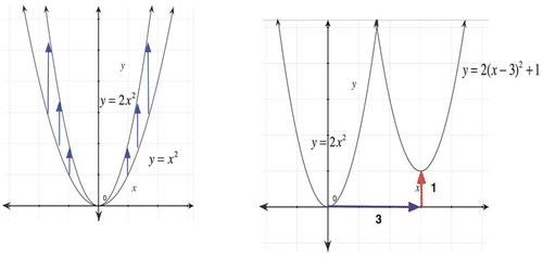
Consider the equation y=2(x−3)2+1. We can compare the graph of this function to the graph of the parent y=x2: the graph represents a vertical stretch by a factor of 2, a horizontal shift 3 units to the right, and a vertical shift of 1 unit.
We can use this relationship to graph the function y=2(x−3)2+1. You can start by sketching y=x2 or y=2x2. Then you can shift the graph 3 units to the right, and up 1 unit.
 [Figure1]
Using your knowledge of the parent function y=|x| and your knowledge of transformations, graph the following function:
f(x)=−|x|+3
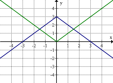
The parent graph of this function is the graph of y=|x|, reflected over the x-axis, and shifted up 3 units. The question is: which transformation do you perform first?
We can answer this question if we consider a few key function values. The table below shows several function values for f(x)=−|x|+3:
| x | f(x)=−abs(x)+3 |
| -3 | −abs(−3)+3=−(+3)+3=−3+3=0 |
| -2 | −abs(−2)+3=−(+2)+3=−2+3=1 |
| -1 | 2 |
| 0 | 3 |
| 1 | 2 |
| 3 | 0 |
From the function values in the table we can see that the function increases until a vertex at (0, 3), and then it decreases again. This tells us that we can obtain the graph if we first reflect y=|x| over the x-axis (turn the “v” upside down), and then shift the graph up 3 units.
 [Figure2]
We can also justify this ordering of the transformations of we think about the order of operations. To find any function value we take an x value, find its absolute value, find the negative of that number, and then add 3. This is the same as the order of the transformation: reflection comes before shifting up.
When describing the relationship between a transformed graph and its parent graph, it is important to be careful with the order of operations. Take the graph of f(x)=3(x+7)3+5 and its parent function g(x)=x3.
The graph of f(x)=4(x+8)3−3 is the graph of g(x)=x3, stretched vertically (made narrower) by a factor of 3, shifted 7 units to the left, and then shifted 5 units up.
Examples
Graph the function below using your knowledge of the parent function y=|x| and your knowledge of transformations.
g(x)=|−x+3|
Solution
This function represents a horizontal shift of y=|x|, and a reflection over the x-axis. Before graphing, consider a few function values:
| x | g(x)=abs(−x+3) |
| -3 | abs(−(−3)+3)=abs(3+3)=abs(6)=6 |
| -2 | abs(−(−2)+3)=(2+3)=abs(5)=5 |
| 0 | 3 |
| 1 | 2 |
| 3 | 0 |
| 4 | 1 |
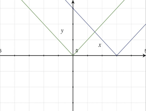
From the values in the table, we can see that the vertex of the graph is at (3, 0). The graph is shown below.
 [Figure3]
The graph looks the same as the graph of y=|x−3|. This is the case because y=|−x+3|=|−(x−3)|, and because |−a|=|a| for all values of a, then |−(x−3)|=|x−3|. So the original function is equal to |x−3|.
We can still think of this graph as a reflection: if we reflect y=|x| over the x-axis, the graph remains the same, as it is symmetric over the x-axis. Then we shift the graph 3 units to the right. What is important to note here is that in order to “read” the equation as a horizontal shift, the entire expression inside the function (in this case, inside the absolute value) must be negated.
Remember that the key to multiple transformations is to do them in order. Another way to keep track of which operations to do in which order is to just do them in the order they appear in the equation, left to right.
Sketch the graph of y=−3(x+2)2+4
Solution
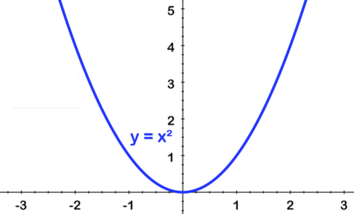
To sketch y=−3(x+2)2+4, we start with the parent function, y=x2.
 [Figure4]
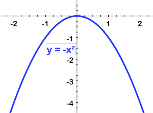 [Figure5]
Next we stretch by 3:
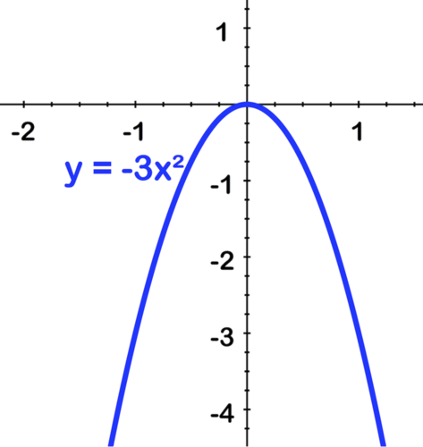 [Figure6]
Shift left by 2:
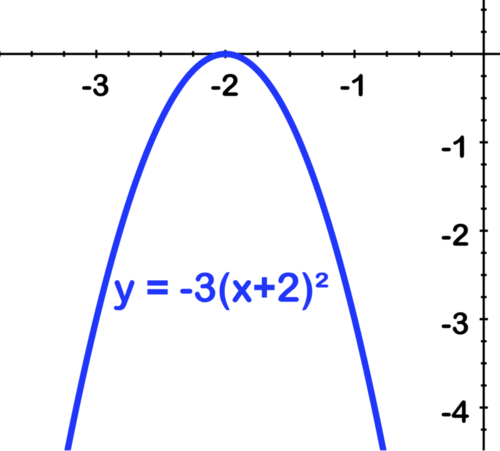 [Figure7]
Finally shift up by 4:
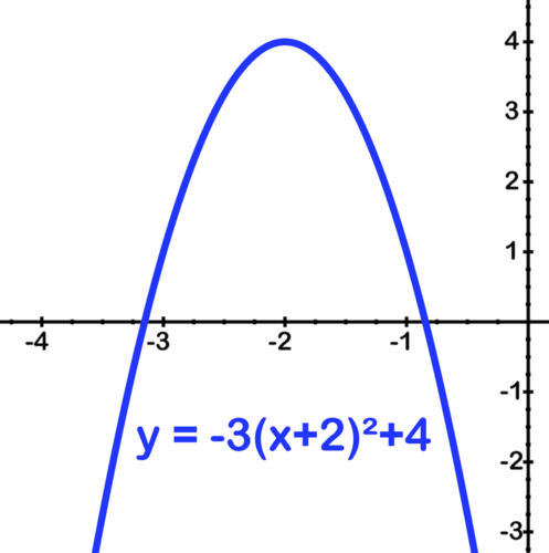 [Figure8]
Sketch the graph of y=−1|x+2|−3
Solution
To sketch y=−1|x+2|−3 start with the parent equation: f(x)=|x| and complete the transformations left to right:
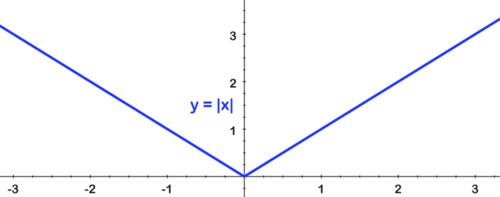 [Figure9]
First reflect over the x axis:
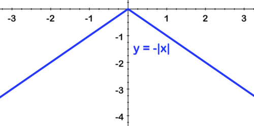 [Figure10]
Second, shift left by 2:
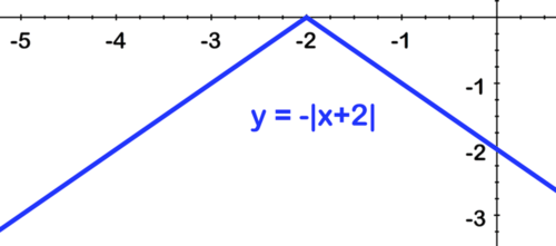 [Figure11]
Finally, shift down by 3:
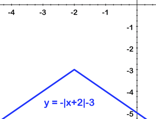 [Figure12]
Sketch the graph of f(x)=2(x−1)2
Solution
To sketch f(x)=2(x−1)2 start with the parent f(x)=x2
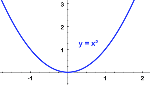 [Figure13]
First stretch by 2:
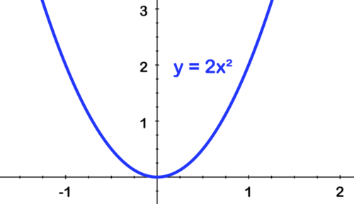 [Figure14]
Second, shift right by 1:
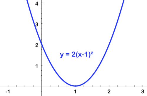 [Figure15]
Sketch the graph of \(\ f(x)=-2 \sqrt{x-1}\)
Solution
To sketch the graph of \(\ f(x)=-2 \sqrt{x-1}\) start with the parent \(\ y=\sqrt{x}\)
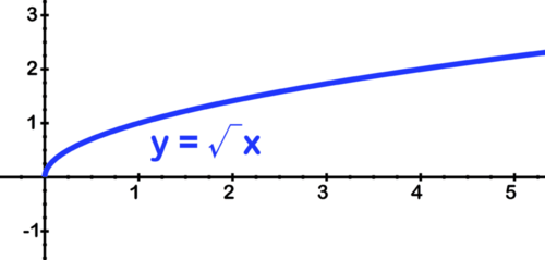 [Figure16]
First reflect over the x axis:
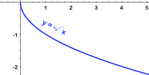 [Figure17]
Second, stretch by 2:
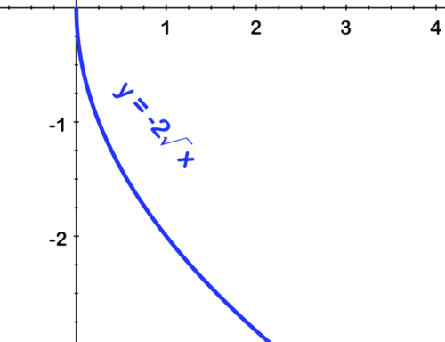 [Figure18]
Third, shift right by 1:
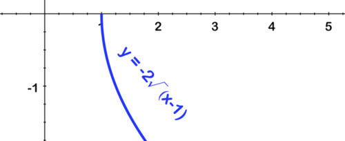 [Figure19]
Review
- What part of the function g(x)=−(f(x)+1)=−(x3+1) shifts the graph of f(x) vertically?
- What part of the function g(x)=−(f(x)+1) reflects the graph of f(x) across the x-axis?
- What is different between the functions g(x)=−(x3+1.0) and h(x)=−x3+1.0 that changes the appearance of the graph?
- Given the function g(x)=3.0(f(x)+2.0)=3.0(x2+2.0), what is it that shifts the graph of f(x) vertically?
- 3.0
- x2
- 2.0
- Given the function g(x)=3.0(f(x)+2.0)=3.0(x2+2.0), what is it that stretches the graph of f(x) vertically?
- 3.0
- x2
- 2.0
- What part of the equation k(x)=−(x+1)3 shifts the graph of j(x)=x3 horizontally?
- What part of the equation k(x)=−(x+1)3 reflects the graph of j(x)=x3 across the x-axis?
- Given the function g(x)=3.0(f(x)+2.0)=3.0(x+2.0)3, what is it that shifts the graph of f(x) horizontally?
- Given the function g(x)=3.0(f(x)+2.0)=3.0(x2+2.0)3, what is it that stretches the graph of f(x) vertically?
- The graph of g(x) is f(x) reflected across the x-axis. The graph of h(x) is f(x) reflected across the y-axis. The graph of j(x) is f(x) reflected across the x-axis and the y-axis. When graphing j(x) does the order in which the reflections occur matter? (Does it matter which axis we reflect the graph across first?)
- Given the function f(x)=x3, write a function g(x) that is: f(x) reflected across the y-axis and then stretched vertically by 8.
- How do you transform the graph of: f(x)=x3 so that it looks like the graph of: f(x)=4x3+6?
- Stretch it by a factor of \(\ 1 \over 4\) and shift it up 6 units.
- Stretch it by a factor of 6 and shift it left 4 units.
- Stretch it by a factor of 4 and shift it down 6 units.
- Stretch it by a factor of 4 and shift it up 6 units.
- How do you transform the graph of: \(\ f(x)=\sqrt{x}\) so that it looks like the graph of: \(\ f(x)=-\sqrt{x}-4\) ?
- Reflect it across the x-axis and shift it 4 units down.
- Reflect it across the y-axis and shift it 4 units up.
- Reflect it across the x-axis and shift it 4 units up.
- Reflect it across the y-axis and shift it 4 units down.
- The graph below is a transformation of a common function. What is the common function that has been transformed?
- y=|x|
- y=\(\ \sqrt{x}\)
- y=x2
- y=x3
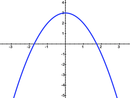 [Figure20]
- How has the function in Q# 14 been transformed?
- Reflected across the y-axis and shifted right 3 units.
- Stretched vertically by a factor of 3 and shifted right 1 unit.
- Reflected across the x-axis and shifted up 3 units.
- Reflected across the x-axis and shifted left 4 units.
- Write a function g(x) whose graph looks like the graph of f(x)=|x| reflected across the x-axis and shifted up 1 unit.
- Choose the function whose graph looks like the graph of f(x)=x3 shifted to the right 2 units and reflected across the y-axis.
- f(x)=(−x−2)3
- f(x)=(−x+2)3
- f(x)=−(x−2)3
- f(x)=(x−2)3
Vocabulary
| Term | Definition |
|---|---|
| parent function | A parent function is the simplest form of a particular type of function. All other functions of this type are usually compared to the parent function. |
| Transformations | Transformations are used to change the graph of a parent function into the graph of a more complex function. |
Image Attributions
- [Figure 1]
License: CC BY-NC-SA - [Figure 2]
License: CC BY-NC-SA - [Figure 3]
License: CC BY-NC-SA - [Figure 4]
License: CC BY-NC-SA - [Figure 5]
License: CC BY-NC-SA - [Figure 6]
License: CC BY-NC-SA - [Figure 7]
License: CC BY-NC-SA - [Figure 8]
License: CC BY-NC-SA - [Figure 9]
Credit: dev Moore;CK-12 Foundation
Source: https://www.flickr.com/photos/devinmoore/187215281/in/photolist-hxwzF-9Y2dT2-8R5iar-9Y2cLM-ePfP1W-eP4pca-epUxUk-ePfP4W-ceh8k3-3dMceZ-aehC8w-gmZd-e3dfr7-ac7c3c-dMr5kM-6bfCWV-6vpzyo-eKFqm1-iEv4o-aYNoV6-aWuFqv-9Uomhm-aWuFb4-eLWJx6-9Y2d4v-aWuFg4-633FZc-7L1mSC-aWuFn6-eKFqkC-7nAuor-9yD6vQ-7jAj2m-aWuFja-bXcHpR-7q9MQ4-eqQMBS-4V9irC-4V9isQ-ePfPis-9mMCH4-7qeaJq-ePfNzy-b3SGm-eP4ok2-eP4oZD-7q9Y2k-ePfP9o-eKFxDm-7qdvyU
License: CC BY-NC-SA - [Figure 10]
Credit: dev Moore;CK-12 Foundation
Source: https://www.flickr.com/photos/devinmoore/187215281/in/photolist-hxwzF-9Y2dT2-8R5iar-9Y2cLM-ePfP1W-eP4pca-epUxUk-ePfP4W-ceh8k3-3dMceZ-aehC8w-gmZd-e3dfr7-ac7c3c-dMr5kM-6bfCWV-6vpzyo-eKFqm1-iEv4o-aYNoV6-aWuFqv-9Uomhm-aWuFb4-eLWJx6-9Y2d4v-aWuFg4-633FZc-7L1mSC-aWuFn6-eKFqkC-7nAuor-9yD6vQ-7jAj2m-aWuFja-bXcHpR-7q9MQ4-eqQMBS-4V9irC-4V9isQ-ePfPis-9mMCH4-7qeaJq-ePfNzy-b3SGm-eP4ok2-eP4oZD-7q9Y2k-ePfP9o-eKFxDm-7qdvyU
License: CC BY-NC-SA - [Figure 11]
Credit: dev Moore;CK-12 Foundation
Source: https://www.flickr.com/photos/devinmoore/187215281/in/photolist-hxwzF-9Y2dT2-8R5iar-9Y2cLM-ePfP1W-eP4pca-epUxUk-ePfP4W-ceh8k3-3dMceZ-aehC8w-gmZd-e3dfr7-ac7c3c-dMr5kM-6bfCWV-6vpzyo-eKFqm1-iEv4o-aYNoV6-aWuFqv-9Uomhm-aWuFb4-eLWJx6-9Y2d4v-aWuFg4-633FZc-7L1mSC-aWuFn6-eKFqkC-7nAuor-9yD6vQ-7jAj2m-aWuFja-bXcHpR-7q9MQ4-eqQMBS-4V9irC-4V9isQ-ePfPis-9mMCH4-7qeaJq-ePfNzy-b3SGm-eP4ok2-eP4oZD-7q9Y2k-ePfP9o-eKFxDm-7qdvyU
License: CC BY-NC-SA - [Figure 12]
Credit: dev Moore;CK-12 Foundation
Source: https://www.flickr.com/photos/devinmoore/187215281/in/photolist-hxwzF-9Y2dT2-8R5iar-9Y2cLM-ePfP1W-eP4pca-epUxUk-ePfP4W-ceh8k3-3dMceZ-aehC8w-gmZd-e3dfr7-ac7c3c-dMr5kM-6bfCWV-6vpzyo-eKFqm1-iEv4o-aYNoV6-aWuFqv-9Uomhm-aWuFb4-eLWJx6-9Y2d4v-aWuFg4-633FZc-7L1mSC-aWuFn6-eKFqkC-7nAuor-9yD6vQ-7jAj2m-aWuFja-bXcHpR-7q9MQ4-eqQMBS-4V9irC-4V9isQ-ePfPis-9mMCH4-7qeaJq-ePfNzy-b3SGm-eP4ok2-eP4oZD-7q9Y2k-ePfP9o-eKFxDm-7qdvyU
License: CC BY-NC-SA - [Figure 13]
License: CC BY-NC-SA - [Figure 14]
License: CC BY-NC-SA - [Figure 15]
License: CC BY-NC-SA - [Figure 16]
License: CC BY-NC-SA - [Figure 17]
License: CC BY-NC-SA - [Figure 18]
License: CC BY-NC-SA - [Figure 19]
License: CC BY-NC-SA - [Figure 20]
License: CC BY-NC-SA

