2.5.2: Polynomial and Rational Inequalities
- Page ID
- 14225
\( \newcommand{\vecs}[1]{\overset { \scriptstyle \rightharpoonup} {\mathbf{#1}} } \)
\( \newcommand{\vecd}[1]{\overset{-\!-\!\rightharpoonup}{\vphantom{a}\smash {#1}}} \)
\( \newcommand{\id}{\mathrm{id}}\) \( \newcommand{\Span}{\mathrm{span}}\)
( \newcommand{\kernel}{\mathrm{null}\,}\) \( \newcommand{\range}{\mathrm{range}\,}\)
\( \newcommand{\RealPart}{\mathrm{Re}}\) \( \newcommand{\ImaginaryPart}{\mathrm{Im}}\)
\( \newcommand{\Argument}{\mathrm{Arg}}\) \( \newcommand{\norm}[1]{\| #1 \|}\)
\( \newcommand{\inner}[2]{\langle #1, #2 \rangle}\)
\( \newcommand{\Span}{\mathrm{span}}\)
\( \newcommand{\id}{\mathrm{id}}\)
\( \newcommand{\Span}{\mathrm{span}}\)
\( \newcommand{\kernel}{\mathrm{null}\,}\)
\( \newcommand{\range}{\mathrm{range}\,}\)
\( \newcommand{\RealPart}{\mathrm{Re}}\)
\( \newcommand{\ImaginaryPart}{\mathrm{Im}}\)
\( \newcommand{\Argument}{\mathrm{Arg}}\)
\( \newcommand{\norm}[1]{\| #1 \|}\)
\( \newcommand{\inner}[2]{\langle #1, #2 \rangle}\)
\( \newcommand{\Span}{\mathrm{span}}\) \( \newcommand{\AA}{\unicode[.8,0]{x212B}}\)
\( \newcommand{\vectorA}[1]{\vec{#1}} % arrow\)
\( \newcommand{\vectorAt}[1]{\vec{\text{#1}}} % arrow\)
\( \newcommand{\vectorB}[1]{\overset { \scriptstyle \rightharpoonup} {\mathbf{#1}} } \)
\( \newcommand{\vectorC}[1]{\textbf{#1}} \)
\( \newcommand{\vectorD}[1]{\overrightarrow{#1}} \)
\( \newcommand{\vectorDt}[1]{\overrightarrow{\text{#1}}} \)
\( \newcommand{\vectE}[1]{\overset{-\!-\!\rightharpoonup}{\vphantom{a}\smash{\mathbf {#1}}}} \)
\( \newcommand{\vecs}[1]{\overset { \scriptstyle \rightharpoonup} {\mathbf{#1}} } \)
\( \newcommand{\vecd}[1]{\overset{-\!-\!\rightharpoonup}{\vphantom{a}\smash {#1}}} \)
\(\newcommand{\avec}{\mathbf a}\) \(\newcommand{\bvec}{\mathbf b}\) \(\newcommand{\cvec}{\mathbf c}\) \(\newcommand{\dvec}{\mathbf d}\) \(\newcommand{\dtil}{\widetilde{\mathbf d}}\) \(\newcommand{\evec}{\mathbf e}\) \(\newcommand{\fvec}{\mathbf f}\) \(\newcommand{\nvec}{\mathbf n}\) \(\newcommand{\pvec}{\mathbf p}\) \(\newcommand{\qvec}{\mathbf q}\) \(\newcommand{\svec}{\mathbf s}\) \(\newcommand{\tvec}{\mathbf t}\) \(\newcommand{\uvec}{\mathbf u}\) \(\newcommand{\vvec}{\mathbf v}\) \(\newcommand{\wvec}{\mathbf w}\) \(\newcommand{\xvec}{\mathbf x}\) \(\newcommand{\yvec}{\mathbf y}\) \(\newcommand{\zvec}{\mathbf z}\) \(\newcommand{\rvec}{\mathbf r}\) \(\newcommand{\mvec}{\mathbf m}\) \(\newcommand{\zerovec}{\mathbf 0}\) \(\newcommand{\onevec}{\mathbf 1}\) \(\newcommand{\real}{\mathbb R}\) \(\newcommand{\twovec}[2]{\left[\begin{array}{r}#1 \\ #2 \end{array}\right]}\) \(\newcommand{\ctwovec}[2]{\left[\begin{array}{c}#1 \\ #2 \end{array}\right]}\) \(\newcommand{\threevec}[3]{\left[\begin{array}{r}#1 \\ #2 \\ #3 \end{array}\right]}\) \(\newcommand{\cthreevec}[3]{\left[\begin{array}{c}#1 \\ #2 \\ #3 \end{array}\right]}\) \(\newcommand{\fourvec}[4]{\left[\begin{array}{r}#1 \\ #2 \\ #3 \\ #4 \end{array}\right]}\) \(\newcommand{\cfourvec}[4]{\left[\begin{array}{c}#1 \\ #2 \\ #3 \\ #4 \end{array}\right]}\) \(\newcommand{\fivevec}[5]{\left[\begin{array}{r}#1 \\ #2 \\ #3 \\ #4 \\ #5 \\ \end{array}\right]}\) \(\newcommand{\cfivevec}[5]{\left[\begin{array}{c}#1 \\ #2 \\ #3 \\ #4 \\ #5 \\ \end{array}\right]}\) \(\newcommand{\mattwo}[4]{\left[\begin{array}{rr}#1 \amp #2 \\ #3 \amp #4 \\ \end{array}\right]}\) \(\newcommand{\laspan}[1]{\text{Span}\{#1\}}\) \(\newcommand{\bcal}{\cal B}\) \(\newcommand{\ccal}{\cal C}\) \(\newcommand{\scal}{\cal S}\) \(\newcommand{\wcal}{\cal W}\) \(\newcommand{\ecal}{\cal E}\) \(\newcommand{\coords}[2]{\left\{#1\right\}_{#2}}\) \(\newcommand{\gray}[1]{\color{gray}{#1}}\) \(\newcommand{\lgray}[1]{\color{lightgray}{#1}}\) \(\newcommand{\rank}{\operatorname{rank}}\) \(\newcommand{\row}{\text{Row}}\) \(\newcommand{\col}{\text{Col}}\) \(\renewcommand{\row}{\text{Row}}\) \(\newcommand{\nul}{\text{Nul}}\) \(\newcommand{\var}{\text{Var}}\) \(\newcommand{\corr}{\text{corr}}\) \(\newcommand{\len}[1]{\left|#1\right|}\) \(\newcommand{\bbar}{\overline{\bvec}}\) \(\newcommand{\bhat}{\widehat{\bvec}}\) \(\newcommand{\bperp}{\bvec^\perp}\) \(\newcommand{\xhat}{\widehat{\xvec}}\) \(\newcommand{\vhat}{\widehat{\vvec}}\) \(\newcommand{\uhat}{\widehat{\uvec}}\) \(\newcommand{\what}{\widehat{\wvec}}\) \(\newcommand{\Sighat}{\widehat{\Sigma}}\) \(\newcommand{\lt}{<}\) \(\newcommand{\gt}{>}\) \(\newcommand{\amp}{&}\) \(\definecolor{fillinmathshade}{gray}{0.9}\)Polynomial and Rational Inequalities
Often it is easier to use and remember new terms when you have a 'hook' or comparison to a term you know already.
"Polynomial inequality" is a term generally used to refer to inequalities where the x variable has a degree of 3 or greater.
The prefix "poly" means 'multiple' or 'many', and the root word "nomial" means 'name' or 'term'.
Therefore a "polynomial" is literally: "many terms".
The prefix "in" means 'not', and the root word "equal" of course means 'the same'.
Therefore and "inequality" refers to things which are "not same" or "not equal".
Can you use this logic to identify the origin of some of the other terms used in this lesson?
Polynomial and Rational Inequalities
Polynomial Inequalities
Solving polynomial inequalities is very similar to solving quadratic inequalities. The basic steps are the same:
- Set up the inequality in the form p(x)>0 (or p(x)<0,p(x)≤0, p(x)≥0)
- Find the solutions to the equation p(x)=0.
- Divide the number line into intervals based on the solutions to p(x)=0.
- Use test points to find solution sets to the equation.
Rational Inequalities
There is one step added to the process of solving rational inequalities because a rational function can also change signs at its vertical asymptotes or at a break in the graph. For instance, look at the graph of the function \(\ r(x)=\frac{x}{x^{2}-9}\) below.
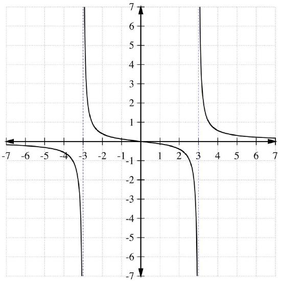
If we want to solve the inequality \(\ \frac{x}{x^{2}-9}>0\), then we need to use the following critical points: x=0,x=3, and x=−3. x=0 is the solution of setting the numerator equal to 0, and this gives us the only root of the function. x=±3 are the vertical asymptotes, the x−coordinates that make the function undefined because putting in 3 or -3 for x will cause a division by zero.
Testing the intervals between each critical point to see if the values in that interval satisfy the function gives us:
| Interval | Test Point | Positive/Negative? | Part of Solution Set? |
|---|---|---|---|
| (−∞,−3) | -4 | - | no |
| (-3, 0) | -2 | + | yes |
| (0, 3) | 2 | - | no |
| (3,+∞) | 4 | + | yes |
Thus, the solutions to \(\ \frac{x}{x^{2}-9}>0\) are x∈(−3,0)∪(3,+∞).
Examples
Earlier, you were given a question about identifying the origins of other terms in this lesson.
Solution
How many of the terms we have used recently were you able to track down the origins of? A few are listed below, did you find others?
Bi-nomial: "two-named" or "two-terms" - from "bi", meaning 'two' and "nomial", meaning 'name' or 'term'. Quad-ratic: "related to a square" - from "quadratus", meaning 'square'. Ratio-nal: "related to a ratio" - from "ratio", meaning 'reason' (as in "to reason" or "calculate") and "-al", meaning "related to".
Solve x3−3x2+2x≥0.
Solution
The polynomial is already in the correct form p(x)≥0 so we solve the equation
x3−3x2+2x=0
x(x2−3x+2)=0
x(x−2)(x−1)=0
The zeros are at x=0,x=1, and x=2.
| Interval | Test Point | Positive/Negative? | Part of Solution Set? |
|---|---|---|---|
| (−∞,0) | -5 | - | no |
| (0, 1) | \(\ 1 \over 2\) | + | yes |
| (1, 2) | \(\ 3 \over 2\) | - | no |
| (2,+∞) | 3 | + | yes |
Notice that this inequality is greater than or equal to zero, so we include the zeros in the solution set. Therefore the solutions are x∈[0,1]∪[2,+∞].
Solve 6x4+5x2<25.
Solution
First we will change the inequality to 6x4+5x2−25<0. Now, solve the equation 6x4+5x2−25=0.
6x4+5x2−25=0
(3x2−5)(2x2+5)=0
The first term yields the solutions \(\ x=\pm \sqrt{\frac{5}{3}}\) and there are no real solutions for the second term.
| Interval | Test Point | Positive/Negative? | Part of Solution Set? |
|---|---|---|---|
| \(\ \left(-\infty,-\sqrt{\frac{5}{3}}\right)\) | -3 | + | no |
| \(\ \left(-\sqrt{\frac{5}{3}}, \sqrt{\frac{5}{3}}\right)\) | 0 | - | yes |
| \(\ \left(\sqrt{\frac{5}{3}},+\infty\right)\) | 3 | + | no |
Finally, the solution set is \(\ x \in\left(-\sqrt{\frac{5}{3}}, \sqrt{\frac{5}{3}}\right)\).
Find the solution set of the inequality
\(\ \frac{4 x-12}{3 x-2}<0\)
Solution
From the numerator we solve 4x−12=0 or x=3. In the denominator, solve 3x−2=0 and we find the critical point \(\ x=frac{2}{3}\).
Making the table
| Interval | Test Point | Positive/Negative? | Part of Solution Set? |
|---|---|---|---|
| \(\ \left(-\infty, \frac{2}{3}\right)\) | 0 | + | no |
| \(\ \left(\frac{2}{3}, 3\right)\) | 1 | - | yes |
| (3,+∞) | 5 | + | no |
Therefore, the solution set includes the numbers in the interval \(\ \left(\frac{2}{3}, 3\right)\). Or in set-builder notation, the solution is \(\ \left\{x \mid \frac{2}{3}<x<3\right\}\).
(using technology) The McNeil Surf Company makes wetsuits. For a given number of wetsuits x, McNeil's profit, in dollars, is given by the function P(x)=−0.01x2+25x−3000.
- If the manager of McNeil wants the profit to stay above $9,000, what is the minimum and maximum number of wetsuits they can manufacture to maintain that level of profit?
- What is the maximum profit McNeil can make?
- Can you explain why this shape might make sense for a profit function?
Solution
- Set up the inequality
−0.01x2 + 25x − 3000 > 9000
−0.01x2 + 25x − 12000 > 0
With a calculator you can graph the function Y1 = −0.01x2 + 25x − 12000.
On a TI-83: use the window [−1000,4000]×[−5000,15000].
The settings are:
Xmin=−1000, Xmax=4000, Xscl=500
Ymin=−5000, Ymax=5000, Yscl=1000 xres=1
On a software grapher, the image looks like this with the window x:0→2400 and y:0→3500
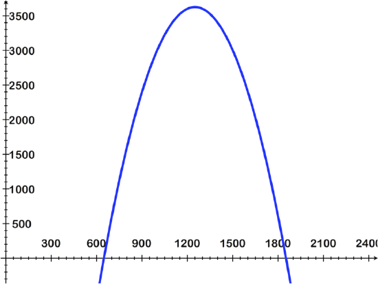
Using the CALC menu (2ND TRACE), and selecting the option ZEROS, we can see that the zeros of Y1=−0.01x2+25x−12000 are at x=647.920 and x=1852.080.
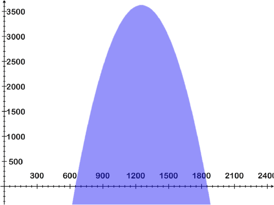
By inspecting the graph, we can see that the solution set to the inequality −0.01x2+25x−12000>0 is x∈(648,1852).
Visually that looks like:
- Keeping the same graph open, use CALC MAXIMUM to solve for the maximum profit. The maximum is at (1250, 3625), indicating that the maximum profit is $3625 above the minimum we set: of $9000.
So the actual maximum profit is $12,625 when 1250 wetsuits are produced.
- One possible reason the profit function might take this shape is labor costs. If McNeil wants to make a very large number of wetsuits in a short period of time, then that may require paying overtime for workers, and this could reduce the profit margin.
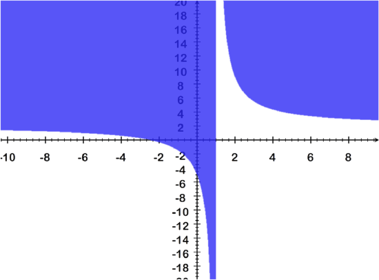
For the following rational function, determine limitations on the domain and the asymptotes, and then sketch the graph.
\(\ f(x) \geq \frac{2 x+5}{x-1}\)
Solution
To identify the graph of the inequality \(\ f(x) \geq \frac{2 x+5}{x-1}\), first treat it as if it were the equality \(\ f(x) \geq \frac{2 x+5}{x-1}\)
For \(\ f(x) \geq \frac{2 x+5}{x-1}\):
To find the critical points, identify the value(s) which make the denominator = 0: x≠1
That gives us a vertical asymptote of x=1
The horizontal asymptote becomes apparent as x becomes truly huge and the "+5" and "-1" no longer matter. At that point, we have \(\ f(x)=\frac{2 x}{x} \rightarrow f(x)=2\) So the horizontal asymptote is y=2
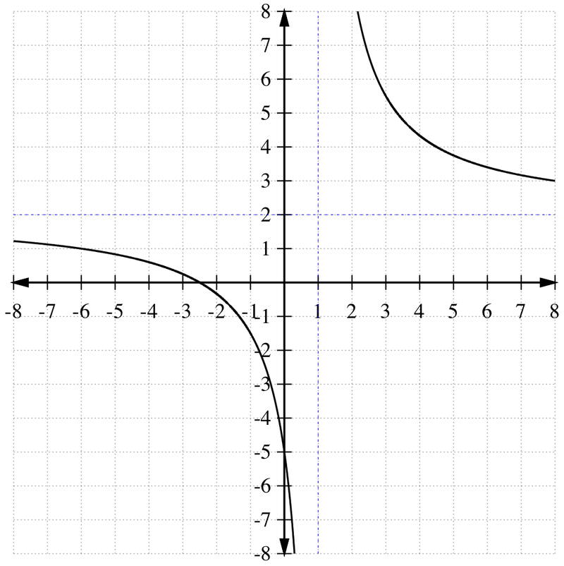
Now that you know the shape of the graph, simply shade the area above the lines, since the original function was f(x) is greater-than function, and leave the lines solid since it was a greater-than or equal to.
The final graph should look like:
Review
Find the solution set of the following inequalities without using a calculator. Display the solution set on a number line.
- x2 + 2x − 3 ≤ 0
- 3x2 − 7x + 2 > 0
- −6x2 − 13x + 5 ≥ 0
- \(\ \frac{5 x-1}{x-2}>0\)
- \(\ \frac{1-x}{x}<1\)
- Solve: 4x3−4x2−3x>0
- Solve: \(\ \frac{x^{4}}{4}-x^{2}<0\)
- Solve: 4x3 − 8x2 − x + 2 ≥ 0
- \(\ \frac{n^{3}-2 n^{2}-n+2}{n^{3}+3 n^{2}+4 n+12}<0\)
- \(\ \frac{n^{3}+3 n^{2}-4 n-12}{n^{3}-5 n^{2}+4 n-20} \leq 0\)
- \(\ \frac{2 n^{3}+5 n^{2}-18 n-45}{3 n^{3}-n^{2}+27 n-9} \geq 0\)
- \(\ \frac{12 n^{3}+16 n^{2}-3 n-4}{8 n^{3}+12 n^{2}+10 n+15}>0\)
Use a calculator to solve the following inequalities. Round your answer to three places after the decimal.
- −9.8t2 + 357.6t ≥ 0
- x3 − 5x + 7 ≤ −4x2 + 18
- \(\ \frac{x^{2}-2 x}{x-5}>x^{2}-25\)
- Solve and graph: \(\ f(x)>\frac{9 x^{2}-4}{3 x+2}\)
- The total resistance of two electronics components wired in parallel is given by \(\ \frac{R_{1} R_{2}}{R_{1}+R_{2}}\) where R1 and R2 are the individual resistances (in Ohms) of the two components. a) If the resistance of R1 is 20 Ohms, what is the maximum resistance of R2 if the total resistance must be less than 15 Ohms? b) What is the maximum theoretical resistance of this circuit? How do you know?
- A rectangular lot of land has a length that is 7 meters more than twice its width. If the area of the lot is greater than 60 square meters, what are the possible values of the widths of the lot?
Vocabulary
| Term | Definition |
|---|---|
| domain | The domain of a function is the set of x-values for which the function is defined. |
| Polynomial inequality | The term polynomial inequality is generally used to describe an inequality with an x term coefficient of three or greater. |
| quadratic inequality | A quadratic inequality is a quadratic expression that is specified to be greater or lesser than a given value. |
| Rational Function | A rational function is any function that can be written as the ratio of two polynomial functions. |
| Rational Inequality | A rational inequality is a ratio of two polynomials, specified to be greater or less than a given value. |
| Vertical Asymptote | A vertical asymptote is a vertical line marking a specific value toward which the graph of a function may approach, but will never reach. |

