2.6.3: Real Zeros of Polynomials

Real Zeros of Polynomials

In the real world, problems do not always easily fit into quadratic or even cubic equations. Financial models, population models, fluid activity, etc., all often require many degrees of the input variable in order to approximate the overall behavior. While it can be challenging to model some of these more complex interactions, the effort can be well worth it. Mathematical models of stocks are used constantly as a way to "look into the future" of finance and make the kinds of educated guesses that are behind some of the largest fortunes in the world.

What benefits can you think of to modeling the behavior of large populations? Can you think of other useful applications not mentioned here?

---

Finding Real Zeros of Polynomials

There are three theorems and a rule that we will be referring to during this lesson in order to help make the discovery of the roots of polynomial functions easier. You should review them and be prepared to refer to them often during the practice problems.

The Remainder Theorem

If a polynomial f(x) of degree n>0 is divided by x−c, then the remainder R is a constant and it is equal to the value of the polynomial when c is substituted for x. That is

f(c)=R

The Factor Theorem

If f(x) is a polynomial of degree n>0 and f(c)=0, then x−c is a factor of the polynomial f(x). Further, if x−c is a factor, then c is a zero of f.

The Rational Zero Theorem

Given the polynomial

f(x)=a_nxⁿ+a_n−1xⁿ⁻¹+⋯+a₁x+a₀

a_n≠0 and n is a positive integer. If the coefficients are integers and \(\ \frac{p}{q}\) is a rational zero in lowest terms, then p is a divisor of a₀ and q is a divisor of a_n.

Descartes' Rule of Signs

Given any polynomial, p(x),

1. Write it with the terms in descending order, i.e. from the highest degree term to the lowest degree term.
2. Count the number of sign changes of the terms in p(x). Call the number of sign changes n.
3. Then the number of positive roots of p(x) is less than or equal to n.
4. Further, the possible number of positive roots is n, n−2, n−4,…
5. To find the number of negative roots of p(x), write p(−x) in descending order as above (i.e. change the sign of all terms in p(x) with odd powers), and repeat the process above. Then the maximum number of negative roots is n.

---

Examples

Example 1

Earlier, you were asked if you could identify some valuable real-world uses for modeling higher-degree polynomials.

Solution

Here are a few possibilities:

• Identifying what times of the day people are most likely to want coffee (market research like this is key to running your own business)
• Predicting population growth in a particular neighborhood or area of town (useful for identifying a good location to start a small business)
• Identifying which stocks are likely to rise or fall based on weather or season
• Forecasting the weather
• Calculating the right head start to give a slower car to make a drag race exciting

There are many, many more.

Example 2

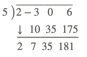
Use synthetic division and the remainder and factor theorems to find the quotient Q(x) and the remainder R if f(x)=2x³−3x²+6 is divided by x−5.

Solution

Hence

2x³−3x²+6=(2x²+7x+35)(x−5)+181

Notice that the remainder is 181 and it can also be obtained if we simply substituted x=5 into f(x),

\(\ \begin{aligned}
f(5) &=2(5)^{3}-3(5)^{2}+6 \\
&=250-75+6 \\
&=181
\end{aligned}\)

Example 3

Use the rational zero theorem and synthetic division to find all the possible rational zeros of the polynomial

f(x)=x³−2x²−x+2

Solution

From the rational zero theorem, \(\ \frac{p}{q}\) is a rational zero of the polynomial f. So p is a divisor of 2 and q is a divisor of 1. Hence, p can take the following values: -1, 1, -2, 2 and q can be either -1 or 1. Therefore, the possible values of \(\ \frac{p}{q}\) are

\(\ \frac{p}{q}:-1,1,-2,2\)

So there are four possible zeros. Of these four, not more than three can be zeros of f because f is a polynomial with degree 3. To test which of the four possible candidates are zeros of f, we use the synthetic division. Recall from the remainder theorem if f(c)=0, then c is a zero of f. We have

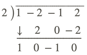
Hence, 2 is a zero of f. Further, by the division algorithm,

\(\ \begin{aligned}
f(x) &=(x-c) Q(x)+R(x) \\
&=(x-2)\left(x^{2}-1\right)+0
\end{aligned}\)

The remaining zeros of f are simply the zeros of Q(x)=x²−1 which is easier to manipulate,

\(\ \begin{aligned}
Q(x) &=x^{2}-1 \\
&=(x-1)(x+1)
\end{aligned}\)

and thus the remaining zeros are -1 and 1. Thus the rational zeros of f are -1, 1, and 2.

Example 4

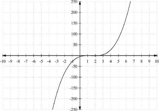
Graph the polynomial function h(x)=2x³−9x²+12x−5.

Solution

Notice that the leading term is 2x³, where n=3 odd and a_n=2>0. This tells us that the end behavior will take the shape of a power function with an odd exponent.

Here, as you can see, there is no straight-forward way to find the zeros of h(x). However, with the use of the factor theorem and the synthetic division, we can find the rational roots of h(x).

First, we use the rational zero theorem and find that the possible rational zeros are

\(\ \frac{p}{q}:-1,1,-2,2,-5,5,-\frac{5}{2}, \frac{5}{2}\)

testing all these numbers by the synthetic division,

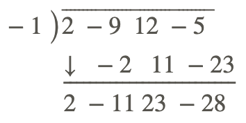
-1 is not a root. Now let's test x=1.

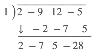
we find that 1 is a zero of h and so we can re-write h(x),

h(x)=(2x²−7x+5)(x−1)

Looking at quadratic part,

2x²−7x+5=(2x−5)(x−1)

and so

h(x)=(2x−5)(x−1)²

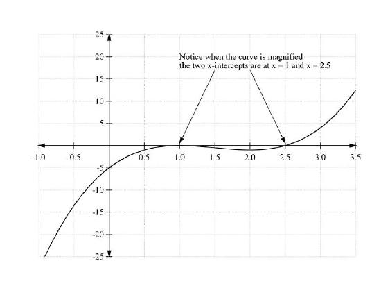
Thus 1 and \(\ \frac{5}{2}\) are the x−intercepts of h(x). The y−intercept is

h(0)=−5

Further, the synthetic division can be also used to form a table of values for the graph of h(x):

x	−1	0	1	2	\(\ \frac{5}{2}\)	3
h(x)	−28	−5	0	-1	0	4

We choose test points from each interval and find g(x).

Interval	Test Value x	h(x)	Sign of h(x)	Location of points on the graph
(−∞, 1)	-1	-28	-	below the x−axis
(1, \(\ \frac{5}{2}\))	\(\ \frac{3}{2}\)	\(\ \frac{-11}{4}\)	-	below the x−axis
(\(\ \frac{5}{2}\), ∞)	3	4	+	above the x−axis

From this information, the graph of h(x) is shown in the two graphs below. Notice that the second graph is a magnification of h(x) in the vicinity of the x−axis.

[Figure1]

[Figure2]

Example 5

Use the 'rational zero' theorem and synthetic division to find all the possible rational zeros of the polynomial

f(x)=x³−2x²−5x+6

Solution

Assume \(\ p\over q\) is a rational zero of f. By the rational zero theorem, p is a divisor of 6 and q is a divisor of 1. Thus p and q can assume the following respective values

p: 1, −1, 2, −2, 3, −3, 6, −6

and

q: −1, 1

Therefore, the possible rational zeros will be

\(\ p\over q\): −1, 1, −2, 2, −3, 3, −6, 6

Notice that with these choices for p and q there could be 8⋅2=16 rational zeros. But, eight of them are duplicates. For example \(\ \frac{1}{-1}=\frac{-1}{1}=-1\). The next step is to test all these values by the synthetic division (we'll let you do this on your own for practice) and we finally find that 1, −2, and 3 are zeros of f. That is

f(x)=x³−2x²−5x+6

=(x−1)(x+2)(x−3)

Example 6

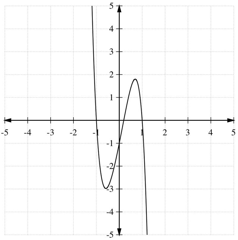
Use Descartes' Rule of Signs to identify the possible number of positive and negative roots of

f(x)=−2x³+x²−3x⁵+5x−1.

Solution

First, re-write f(x) in descending order

f(x)=−3x⁵−2x³+x²+5x−1.

The number of sign changes of f(x) is 2, so the number of positive roots is either 2 or 0.

For the negative roots, write

f(−x)=−3x⁵+2x³+x²−5x−1

The number of sign changes of f(−x) is 2, so the maximum number of negative roots is 2.

The graph of f(x) below shows that there is one negative root and two positive roots.

[Figure3]

---

Review

Questions 1 - 3: Use a) long division and b) synthetic division to perform the divisions. Express each result in the form: f(x)=D(x)⋅Q(x)+R.

1. 5x⁵ − 3x⁴ + 2x³ + x² − 7x + 3 by x−2
2. −4x⁶ − 5x³ + 3x² + x + 7 by x−1
3. 2x³ − 5x² + 5x + 11 by x -\(\ \frac{1}{2}\)
4. Use synthetic division to find Q(x) and f(c) so that f(x)=(x−c)Q(x)+f(c) if f(x) = −3x⁴ − 3x³ + 3x² + 2x − 4 and c = −2
5. If f(x) = x³ + 2x² − 10x + 10, use synthetic division to determine the following: a) f(−1) b) f(−3) c) f(0) d) f(4) e) What are the factors of f(x)?
6. Find k so that x−2 is a factor of f(x) = 3x³ + 4x² + kx − 20
7. Use synthetic division to determine all the zeros of the polynomials: a) f(x) = 3x³ − 7x² + 8x − 2 b) g(x) = 4x⁴ − 4x³ − 7x² + 4x + 3
8. Graph the polynomial function f(x) = x³ − 2x² − 5x + 6 by using synthetic division to find the x−intercepts and locate the y−intercepts.
9. Graph the polynomial function h(x)= x³ − 3x² + 4 by using synthetic division to find the x−intercepts and locate the y−intercepts.
10. Write a 3rd degree equation of a polynomial function with the zeroes: 0, 2, and -5.
11. Write a 7th degree equation of a polynomial function with the zeroes: 0 (multiplicity 2), 2 (multiplicity 3), and -5 (multiplicity 2)
12. Write a quadratic equation which has 4 (multiplicity 2) as the zero and opens downward.
13. Write a 3rd degree polynomial function with the zeroes: -2, 2, and 6, passing through the point (3, 4)
14. Let f(x) = 2x³ − 5x² − 4x + 3 and find the solutions: a) f(x)=0 b) f(2x)=0
15. Graph and find the solution set of the inequality x³ − 2x² − 5x + 6 ≤ 0.
16. Use the graph of f(x)=x(x−1)(x+2) to find the solution set of the inequality x(x−1)(x+2)>0.

---

Review (Answers)

To see the Review answers, open this PDF file and look for section 2.12.

---

Vocabulary

Term	Definition
Descartes' Rule of Signs	Descartes' rule of signs is a technique for determining the number of positive and negative real roots of a polynomial.
factor theorem	The factor theorem states that if f(x) is a polynomial of degree n>0 and f(c)=0, then x−c is a factor of the polynomial f(x).
factorization theorem	The factorization theorem states that If f(x) = anx^n+ an−1x^n−1+ ⋯ + a1x + a0, where an≠0, and n is a positive integer, then f(x) = an(x−c1)(x−c2)⋯(x−c0) where the numbers ci are complex numbers.
Multiplicity	The multiplicity of a term describes the number of times the given term acts as a zero of the given function.
Polynomial	A polynomial is an expression with at least one algebraic term, but which does not indicate division by a variable or contain variables with fractional exponents.
Rational Zero Theorem	The rational zero theorem states that for a polynomial, f(x) = anx^n+ an−1x^n−1+ ⋯ + a1x + a0, where an, an−1,⋯ a0 are integers, the rational roots can be determined from the factors of an and a0. More specifically, if p is a factor of a0 and q is a factor of an, then all the rational factors will have the form \(\ \pm \frac{p}{q}\).
Remainder Theorem	The remainder theorem states that if f(k)=r, then r is the remainder when dividing f(x) by (x−k).
Roots	The roots of a function are the values of x that make y equal to zero.
Synthetic Division	Synthetic division is a shorthand version of polynomial long division where only the coefficients of the polynomial are used.
Zeroes	The zeroes of a function f(x) are the values of x that cause f(x) to be equal to zero.
Zeros	The zeros of a function f(x) are the values of x that cause f(x) to be equal to zero.

---

Image Attributions

1. [Figure 1]
   Credit: CK-12
   Source: CK-12
2. [Figure 2]
   Credit: CK-12
   Source: CK-12
3. [Figure 3]
   Credit: CK-12
   Source: CK-12