2.6.2: Synthetic Division of Polynomials

Synthetic Division of Polynomials

The volume of a rectangular prism is 2x³+5x²−x−6. Determine if 2x+3 is the length of one of the prism's sides.

---

Synthetic Division

Synthetic division is an alternative to long division. It can also be used to divide a polynomial by a possible factor, x−k. However, synthetic division cannot be used to divide larger polynomials, like quadratics, into another polynomial.

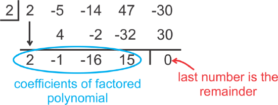
Let's use synthetic division to divide 2x⁴−5x³−14x²+47x−30 by x−2.

Using synthetic division, the setup is as follows:

[Figure1]

[Figure2]

[Figure3]

[Figure4]

[Figure5]

To “read” the answer, use the numbers as follows:

[Figure6]

Therefore, 2 is a solution, because the remainder is zero. The factored polynomial is 2x³−x²−16x+15. Notice that when we synthetically divide by k, the “leftover” polynomial is one degree less than the original. We could also write

(x−2)(2x³−x²−16x+15)=2x⁴−5x³−14x²+47x−30.

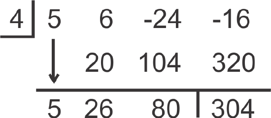
Now, let's determine if 4 is a solution to f(x)=5x³+6x²−24x−16.

Using synthetic division, we have:

[Figure7]

The remainder is 304, so 4 is not a solution. Notice if we substitute in x=4, also written f(4), we would have f(4)=5(4)³+6(4)²−24(4)−16=304. This leads us to the Remainder Theorem.

Remainder Theorem: If f(k)=r, then r is also the remainder when dividing by (x−k).

This means that if you substitute in x=k or divide by k, what comes out of f(x) is the same. r is the remainder, but it is also the corresponding y−value. Therefore, the point (k,r) would be on the graph of f(x).

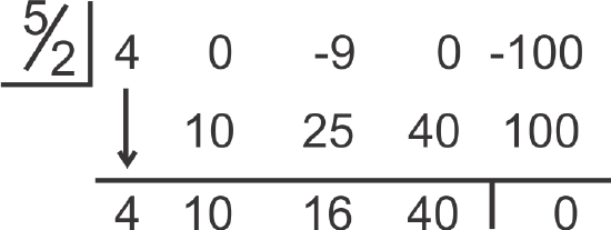
Finally, let's determine if (2x−5) is a factor of 4x⁴−9x²−100.

If you use synthetic division, the factor is not in the form (x−k). We need to solve the possible factor for zero to see what the possible solution would be. Therefore, we need to put \(\ \frac{5}{2}\) up in the left-hand corner box. Also, not every term is represented in this polynomial. When this happens, you must put in zero placeholders. In this problem, we need zeros for the x³−term and the x−term.

[Figure8]

This means that \(\ \frac{5}{2}\) is a zero and its corresponding binomial, (2x−5), is a factor.

---

Example 1

Earlier, you were asked to determine if 2x+3 is the length of one of the prism's sides.

Solution

If 2x+3 divides evenly into 2x³+5x²−x−6 then it is the length of one of the prism's sides.

If we want to use synthetic division, notice that the factor is not in the form (x−k). Therefore, we need to solve the possible factor for zero to see what the possible solution would be. If 2x+3=0 then x=\(\ -\frac{3}{2}\). Therefore, we need to put \(\ -\frac{3}{2}\) up in the left-hand corner box.

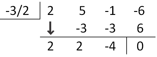
When we perform the synthetic division, we get a remainder of 0. This means that (2x+3) is a factor of the volume. Therefore, it is also the length of one of the sides of the rectangular prism.

Example 2

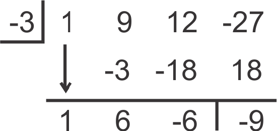
Divide x³+9x²+12x−27 by (x+3). Write the resulting polynomial with the remainder (if there is one).

Solution

Using synthetic division, divide by -3.

[Figure9]

The answer is \(\ x^{2}+6 x-6-\frac{9}{x+3}\).

Example 3

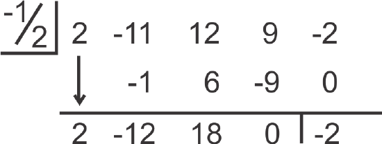
Divide 2x⁴−11x³+12x²+9x−2 by (2x+1). Write the resulting polynomial with the remainder (if there is one).

Solution

Using synthetic division, divide by \(\ -\frac{1}{2}\).

[Figure10]

The answer is \(\ 2 x^{3}-12 x^{2}+18 x-\frac{2}{2 x+1}\)

Example 4

Is 6 a solution for f(x)=x³−8x²+72? If so, find the real-number zeros (solutions) of the resulting polynomial.

Solution

Put a zero placeholder for the x−term. Divide by 6.

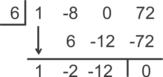
The resulting polynomial is x²−2x−12. While this quadratic does not factor, we can use the Quadratic Formula to find the other roots.

\(\ x=\frac{2 \pm \sqrt{2^{2}-4(1)(-12)}}{2}=\frac{2 \pm \sqrt{4+48}}{2}=\frac{2 \pm 2 \sqrt{13}}{2}=1 \pm \sqrt{13}\)

The solutions to this polynomial are \(\ 6,1+\sqrt{13} \approx 4.61 \text { and } 1-\sqrt{13} \approx-2.61\).

---

Review

Use synthetic division to divide the following polynomials. Write out the remaining polynomial.

1. (x³+6x²+7x+10)÷(x+2)
2. (4x³−15x²−120x−128)÷(x−8)
3. (4x²−5)÷(2x+1)
4. (2x⁴−15x³−30x²−20x+42)÷(x+9)
5. (x³−3x²−11x+5)÷(x−5)
6. (3x⁵+4x³−x−2)÷(x−1)
7. Which of the division problems above generate no remainder? What does that mean?
8. What is the difference between a zero and a factor?
9. Find f(−2) if f(x)=2x⁴−5x³−10x²+21x−4.
10. Now, divide 2x⁴−5x³−10x²+21x−4 by (x+2) synthetically. What do you notice?

Find all real zeros of the following polynomials, given one zero.

11. 12x³+76x²+107x−20; −4
12. x³−5x²−2x+10; −2
13. 6x³−17x²+11x−2; 2

Find all real zeros of the following polynomials, given two zeros.

14. x⁴+7x³+6x²−32x−32; −4, −1
15. 6x⁴+19x³+11x²−6x; 0, −2

---

Answers for Review Problems

To see the Review answers, open this PDF file and look for section 6.10.

---

Vocabulary

Term	Definition
Oblique Asymptote	An oblique asymptote is a diagonal line marking a specific range of values toward which the graph of a function may approach, but generally never reach. An oblique asymptote exists when the numerator of the function is exactly one degree greater than the denominator. An oblique asymptote may be found through long division.
Oblique Asymptotes	An oblique asymptote is a diagonal line marking a specific range of values toward which the graph of a function may approach, but generally never reach. An oblique asymptote exists when the numerator of the function is exactly one degree greater than the denominator. An oblique asymptote may be found through long division.
Remainder Theorem	The remainder theorem states that if f(k)=r, then r is the remainder when dividing f(x) by (x−k).
Synthetic Division	Synthetic division is a shorthand version of polynomial long division where only the coefficients of the polynomial are used.

---

Image Attributions

1. [Figure 1]
   Credit: CK-12 Foundation
   Source: http://centros5.pntic.mec.es/sierrami/dematesna/demates67/opciones/sabias/Ruffinni/Ruffinni.htm
2. [Figure 2]
   Credit: CK-12 Foundation
   Source: http://centros5.pntic.mec.es/sierrami/dematesna/demates67/opciones/sabias/Ruffinni/Ruffinni.htm
3. [Figure 3]
   Credit: CK-12 Foundation
   Source: http://centros5.pntic.mec.es/sierrami/dematesna/demates67/opciones/sabias/Ruffinni/Ruffinni.htm
4. [Figure 4]
   Credit: CK-12 Foundation
   Source: http://centros5.pntic.mec.es/sierrami/dematesna/demates67/opciones/sabias/Ruffinni/Ruffinni.htm
5. [Figure 5]
   Credit: CK-12 Foundation
   Source: http://centros5.pntic.mec.es/sierrami/dematesna/demates67/opciones/sabias/Ruffinni/Ruffinni.htm
6. [Figure 6]
   Credit: CK-12 Foundation
   Source: http://centros5.pntic.mec.es/sierrami/dematesna/demates67/opciones/sabias/Ruffinni/Ruffinni.htm
7. [Figure 7]
   Credit: CK-12 Foundation
   Source: http://centros5.pntic.mec.es/sierrami/dematesna/demates67/opciones/sabias/Ruffinni/Ruffinni.htm
8. [Figure 8]
   Credit: CK-12 Foundation
   Source: http://centros5.pntic.mec.es/sierrami/dematesna/demates67/opciones/sabias/Ruffinni/Ruffinni.htm
9. [Figure 9]
   Credit: CK-12 Foundation
   Source: http://centros5.pntic.mec.es/sierrami/dematesna/demates67/opciones/sabias/Ruffinni/Ruffinni.htm
10. [Figure 10]
    Credit: CK-12 Foundation
    Source: http://centros5.pntic.mec.es/sierrami/dematesna/demates67/opciones/sabias/Ruffinni/Ruffinni.htm