8.4.1: Area Under the Curve
- Page ID
- 14824
\( \newcommand{\vecs}[1]{\overset { \scriptstyle \rightharpoonup} {\mathbf{#1}} } \)
\( \newcommand{\vecd}[1]{\overset{-\!-\!\rightharpoonup}{\vphantom{a}\smash {#1}}} \)
\( \newcommand{\dsum}{\displaystyle\sum\limits} \)
\( \newcommand{\dint}{\displaystyle\int\limits} \)
\( \newcommand{\dlim}{\displaystyle\lim\limits} \)
\( \newcommand{\id}{\mathrm{id}}\) \( \newcommand{\Span}{\mathrm{span}}\)
( \newcommand{\kernel}{\mathrm{null}\,}\) \( \newcommand{\range}{\mathrm{range}\,}\)
\( \newcommand{\RealPart}{\mathrm{Re}}\) \( \newcommand{\ImaginaryPart}{\mathrm{Im}}\)
\( \newcommand{\Argument}{\mathrm{Arg}}\) \( \newcommand{\norm}[1]{\| #1 \|}\)
\( \newcommand{\inner}[2]{\langle #1, #2 \rangle}\)
\( \newcommand{\Span}{\mathrm{span}}\)
\( \newcommand{\id}{\mathrm{id}}\)
\( \newcommand{\Span}{\mathrm{span}}\)
\( \newcommand{\kernel}{\mathrm{null}\,}\)
\( \newcommand{\range}{\mathrm{range}\,}\)
\( \newcommand{\RealPart}{\mathrm{Re}}\)
\( \newcommand{\ImaginaryPart}{\mathrm{Im}}\)
\( \newcommand{\Argument}{\mathrm{Arg}}\)
\( \newcommand{\norm}[1]{\| #1 \|}\)
\( \newcommand{\inner}[2]{\langle #1, #2 \rangle}\)
\( \newcommand{\Span}{\mathrm{span}}\) \( \newcommand{\AA}{\unicode[.8,0]{x212B}}\)
\( \newcommand{\vectorA}[1]{\vec{#1}} % arrow\)
\( \newcommand{\vectorAt}[1]{\vec{\text{#1}}} % arrow\)
\( \newcommand{\vectorB}[1]{\overset { \scriptstyle \rightharpoonup} {\mathbf{#1}} } \)
\( \newcommand{\vectorC}[1]{\textbf{#1}} \)
\( \newcommand{\vectorD}[1]{\overrightarrow{#1}} \)
\( \newcommand{\vectorDt}[1]{\overrightarrow{\text{#1}}} \)
\( \newcommand{\vectE}[1]{\overset{-\!-\!\rightharpoonup}{\vphantom{a}\smash{\mathbf {#1}}}} \)
\( \newcommand{\vecs}[1]{\overset { \scriptstyle \rightharpoonup} {\mathbf{#1}} } \)
\(\newcommand{\longvect}{\overrightarrow}\)
\( \newcommand{\vecd}[1]{\overset{-\!-\!\rightharpoonup}{\vphantom{a}\smash {#1}}} \)
\(\newcommand{\avec}{\mathbf a}\) \(\newcommand{\bvec}{\mathbf b}\) \(\newcommand{\cvec}{\mathbf c}\) \(\newcommand{\dvec}{\mathbf d}\) \(\newcommand{\dtil}{\widetilde{\mathbf d}}\) \(\newcommand{\evec}{\mathbf e}\) \(\newcommand{\fvec}{\mathbf f}\) \(\newcommand{\nvec}{\mathbf n}\) \(\newcommand{\pvec}{\mathbf p}\) \(\newcommand{\qvec}{\mathbf q}\) \(\newcommand{\svec}{\mathbf s}\) \(\newcommand{\tvec}{\mathbf t}\) \(\newcommand{\uvec}{\mathbf u}\) \(\newcommand{\vvec}{\mathbf v}\) \(\newcommand{\wvec}{\mathbf w}\) \(\newcommand{\xvec}{\mathbf x}\) \(\newcommand{\yvec}{\mathbf y}\) \(\newcommand{\zvec}{\mathbf z}\) \(\newcommand{\rvec}{\mathbf r}\) \(\newcommand{\mvec}{\mathbf m}\) \(\newcommand{\zerovec}{\mathbf 0}\) \(\newcommand{\onevec}{\mathbf 1}\) \(\newcommand{\real}{\mathbb R}\) \(\newcommand{\twovec}[2]{\left[\begin{array}{r}#1 \\ #2 \end{array}\right]}\) \(\newcommand{\ctwovec}[2]{\left[\begin{array}{c}#1 \\ #2 \end{array}\right]}\) \(\newcommand{\threevec}[3]{\left[\begin{array}{r}#1 \\ #2 \\ #3 \end{array}\right]}\) \(\newcommand{\cthreevec}[3]{\left[\begin{array}{c}#1 \\ #2 \\ #3 \end{array}\right]}\) \(\newcommand{\fourvec}[4]{\left[\begin{array}{r}#1 \\ #2 \\ #3 \\ #4 \end{array}\right]}\) \(\newcommand{\cfourvec}[4]{\left[\begin{array}{c}#1 \\ #2 \\ #3 \\ #4 \end{array}\right]}\) \(\newcommand{\fivevec}[5]{\left[\begin{array}{r}#1 \\ #2 \\ #3 \\ #4 \\ #5 \\ \end{array}\right]}\) \(\newcommand{\cfivevec}[5]{\left[\begin{array}{c}#1 \\ #2 \\ #3 \\ #4 \\ #5 \\ \end{array}\right]}\) \(\newcommand{\mattwo}[4]{\left[\begin{array}{rr}#1 \amp #2 \\ #3 \amp #4 \\ \end{array}\right]}\) \(\newcommand{\laspan}[1]{\text{Span}\{#1\}}\) \(\newcommand{\bcal}{\cal B}\) \(\newcommand{\ccal}{\cal C}\) \(\newcommand{\scal}{\cal S}\) \(\newcommand{\wcal}{\cal W}\) \(\newcommand{\ecal}{\cal E}\) \(\newcommand{\coords}[2]{\left\{#1\right\}_{#2}}\) \(\newcommand{\gray}[1]{\color{gray}{#1}}\) \(\newcommand{\lgray}[1]{\color{lightgray}{#1}}\) \(\newcommand{\rank}{\operatorname{rank}}\) \(\newcommand{\row}{\text{Row}}\) \(\newcommand{\col}{\text{Col}}\) \(\renewcommand{\row}{\text{Row}}\) \(\newcommand{\nul}{\text{Nul}}\) \(\newcommand{\var}{\text{Var}}\) \(\newcommand{\corr}{\text{corr}}\) \(\newcommand{\len}[1]{\left|#1\right|}\) \(\newcommand{\bbar}{\overline{\bvec}}\) \(\newcommand{\bhat}{\widehat{\bvec}}\) \(\newcommand{\bperp}{\bvec^\perp}\) \(\newcommand{\xhat}{\widehat{\xvec}}\) \(\newcommand{\vhat}{\widehat{\vvec}}\) \(\newcommand{\uhat}{\widehat{\uvec}}\) \(\newcommand{\what}{\widehat{\wvec}}\) \(\newcommand{\Sighat}{\widehat{\Sigma}}\) \(\newcommand{\lt}{<}\) \(\newcommand{\gt}{>}\) \(\newcommand{\amp}{&}\) \(\definecolor{fillinmathshade}{gray}{0.9}\)Area Under a Curve
Calculating the area under a straight line can be done with geometry. Calculating the area under a curved line requires calculus. Often the area under a curve can be interpreted as the accumulated amount of whatever the function is modeling. Suppose a car’s speed in meters per second can be modeled by a quadratic for the first 8 seconds of acceleration:
\(\ s(t)=t^{2}\)
How far has the car traveled in 8 seconds?
Finding the Area Under a Curve
The area under a curve can be approximated with rectangles equally spaced under a curve as shown below. For consistency, you can choose whether the boxes should hit the curve on the left hand corner, the right hand corner, the maximum value, or the minimum value. The more boxes you use the narrower the boxes will be and thus, the more accurate your approximation of the area will be.
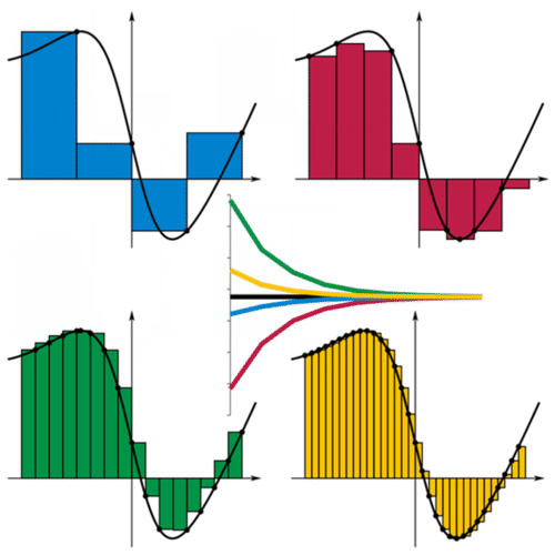
Subintervals are created when an interval is broken into smaller, equally sized intervals. The blue approximation uses right handed boxes for the height of each subinterval. The red approximation assigns the height of the box to be the minimum value of the function in each subinterval. The green approximation assigns the height of the box to be the maximum value of the function in each subinterval. The yellow approximation uses left handed boxes. Rectangles above the x-axis will have positive area and rectangles below the x-axis will have negative area in this context.
Using boxes to estimate the area under a curve is called a Riemann Sum. Take the function \(\ f(x)=\frac{1}{2} x-2\). To calculate the Riemann Sum (area under the curve) between 1 and 9 of the function, first draw the graph and the boxes.
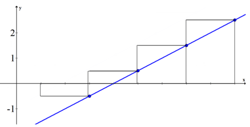
The area of the first box is 2 times the height of the function evaluated at 3:
\(\ 2 \cdot\left(\frac{1}{2} \cdot 3-2\right)=3-4=-1\)
Because this box is under the x-axis, its area is negative.
The area for each of the rest of the boxes is 2 times the height of the function evaluated at 5, 7 and 9.
\(\ \begin{array}{l}
2 \cdot\left(\frac{1}{2} \cdot 5-2\right)&=5-4=1 \\
2 \cdot\left(\frac{1}{2} \cdot 7-2\right)&=7-4=3 \\
2 \cdot\left(\frac{1}{2} \cdot 9-2\right)&=9-4=5
\end{array}\)
The approximate sum of the total area under the curve is: −1+1+3+5=8 square units.
All four of the area approximations shown earlier get better as the number of boxes increase. In fact, the limit of each approximation as the number of subintervals(boxes) increases to infinity is the precise area under the curve.
This is where the calculus idea of an integral comes in. An integral is the limit of a sum as the number of summands increases to infinity. A summand is one of many pieces being summed together.
\(\ \int f(x)=\lim _{n \rightarrow \infty} \sum_{i=1}^{n}(\text { Area of box } i)\)
The symbol on the left is the calculus symbol of an integral.
Examples
Earlier, you were asked to determine how far a car travels in 8 seconds.
Solution
You can use the area under the curve to find the total distance traveled in the first 8 seconds. Since the quadratic is a curve you must choose the number of subintervals you want to use and whether you want right or left handed boxes for estimating. Suppose you choose 8 left handed boxes of width one.
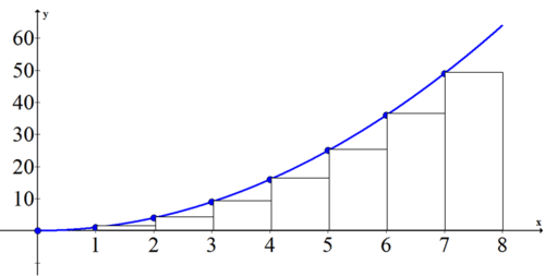
| x | 0 | 1 | 2 | 3 | 4 | 5 | 6 | 7 |
| Area of box to the right | 1⋅0 | 1⋅1 | 1⋅4 | 1⋅9 | 1⋅16 | 1⋅25 | 1⋅36 | 1⋅49 |
The approximate sum is 1+4+9+16+25+36+49=140. This means that the car traveled approximately 140 meters in the first 8 seconds.
Evaluate the exact area under the curve used earlier, \(\ f(x)=\frac{1}{2} x-2\), using the area formula for a triangle.
Solution
Remember that the area below the \(\ x\) axis is negative while the area above the \(\ x\) axis is positive.
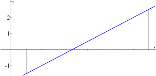
Negative Area: \(\ \frac{1}{2} \cdot 3 \cdot 1.5=\frac{9}{4}\)
Positive Area: \(\ \frac{1}{2} \cdot 5 \cdot 2.5=\frac{25}{4}\)
Area under the curve between 1 and 8: \(\ \frac{25}{4}-\frac{9}{4}=\frac{16}{4}=4\)
If you compare this answer to the approximation from earlier, it appears that approximations that are 2 units wide produce an area with significant error.
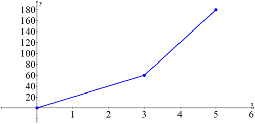
Logan travels by bike at 20 mph for 3 hours. Then she gets in a car and drives 60 mph for 2 hours. Sketch both the distance vs. time graph and the rate vs. time graph. Use an area under the curve argument to connect the two graphs.
Solution
Distance vs. Time:
Rate vs. Time:
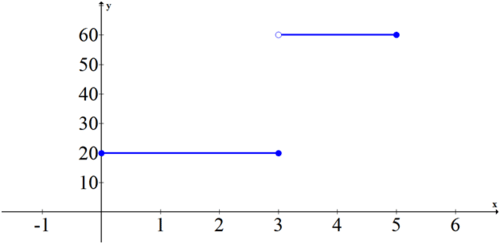
The slope of the first graph is 20 from 0 to 3 and then 60 from 3 to 5. The second graph is a graph of the slopes from the first graph. If you calculate the area of the second graph at the key points 0, 1, 2, 3, 4 and 5 you will see that they align perfectly with the points on the first graph.
| x | Area under curve from 0 to x |
| 0 | 0 |
| 1 | 20 |
| 2 | 40 |
| 3 | 60 |
| 4 | 120 |
| 5 | 180 |
Approximate the area under the curve using eight subintervals and right endpoints.
\(\ f(x)=3 x^{2}-1,-1 \leq x \leq 7\)
Solution
While a graph is helpful to visualize the problem and drawing each box can help give meaning to each summand, it is not always necessary. Since there are going to be 8 subintervals over the total interval of −1≤x≤7, each interval is going to have a width of 1. The height of each interval is going to be at the right hand endpoints of each subinterval (0, 1, 2, 3, 4, 5, 6, 7).
\(\ \sum \text { height } \cdot \text { width }=\sum_{i=0}^{7}\left(3 i^{2}-1\right) \cdot 1=412\)
Approximate the area under the curve using twenty subintervals and left endpoints.
\(\ f(x)=x^{x}, 1 \leq x \leq 3\)
Solution
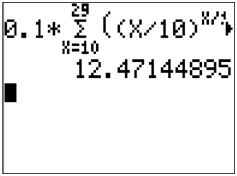
When the number of subintervals gets large and the subintervals get extremely narrow it will be impossible to draw an accurate picture. This is why using summation notation and thinking through what the indices and the argument will be is incredibly important. With 20 subintervals between [1,3], each interval will be 0.1 wide. Left endpoints means that the first box has a height of \(\ f(1)\) and the second box has a height of \(\ f(1.1)\).
\(\ \begin{aligned}
\sum \text { height } \cdot \text { width } &=f(1) \cdot 0.1+f(1.1) \cdot 0.1+f(1.2) \cdot 0.1+\cdots+f(2.9) \cdot 0.1 \\
&=0.1(f(1)+f(1.1)+\cdots f(2.9)) \\
&=0.1 \cdot \sum_{i=10}^{29} f\left(\frac{i}{10}\right) \\
&=0.1 \cdot \sum_{i=10}^{29}\left(\frac{i}{10}\right)^{\left(\frac{i}{10}\right)} \\
& \approx 12.47144
\end{aligned}\)
Your calculator can compute summations when you go under the math menu.
Review
- Approximate the area under the curve using eight subintervals and right endpoints.
\(\ f(x)=x^{2}-x+1,0 \leq x \leq 8\)
- Approximate the area under the curve using eight subintervals and left endpoints.
\(\ f(x)=x^{2}-2 x+1,-4 \leq x \leq 4\)
- Approximate the area under the curve using twenty subintervals and left endpoints.
\(\ f(x)=\sqrt{x+3}, 0 \leq x \leq 4\)
- Approximate the area under the curve using 100 subintervals and left endpoints. Compare to your answer from #3.
\(\ f(x)=\sqrt{x+3}, 0 \leq x \leq 4\)
- Approximate the area under the curve using eight subintervals and left endpoints.
\(\ f(x)=\cos (x), 0 \leq x \leq 4\)
- Approximate the area under the curve using twenty subintervals and left endpoints.
\(\ f(x)=\cos (x), 0 \leq x \leq 4\)
- Approximate the area under the curve using 100 subintervals and left endpoints.
\(\ f(x)=\cos (x), 0 \leq x \leq 4\)
The following graph shows the rate (in miles per hour) vs. time (in hours) for a car.
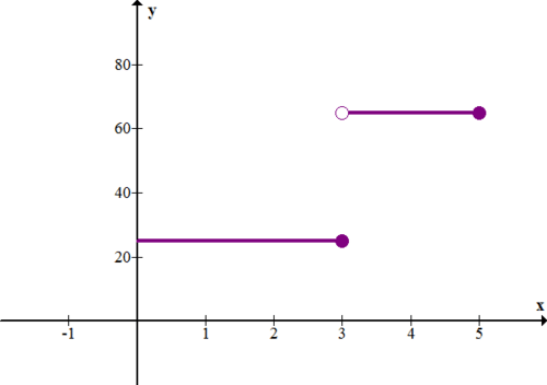
8. Describe what is happening with the car.
9. How far did the car travel in 5 hours?
The following graph shows the rate (in feet per second) vs. time (in seconds) for a car.
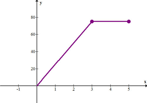
10. Describe what is happening with the car. In particular, what is happening in the first 3 seconds?
11. How far did the car travel in 5 seconds?
The following graph shows the function \(\ f(x)=-(x-4)^{2}+16\), which represents the rate (in feet per second) vs. time (in seconds) for a runner.
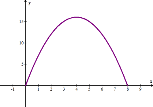
12. Describe what is happening with the runner. In particular, what happens after 4 seconds?
13. Use rectangles to approximate the total distance (in feet) that the runner traveled in the 8 seconds. Try to get as good an approximation as possible.
14. Explain how an integral is like the opposite of a derivative.
15. How do integrals relate to sums?
Vocabulary
| Term | Definition |
|---|---|
| Δ | The symbol "Δ", read "delta", is used to denote "change in", as in "the change in velocity over time" \(\ =\frac{\Delta v}{t}\). |
| definite integral | A definite integral gives the area between the x-axis and a curve over a defined interval. |
| limit | A limit is the value that the output of a function approaches as the input of the function approaches a given value. |
| subintervals | Subintervals are created when an interval is broken into smaller equally sized intervals. |
| summand | A summand is an expression being summed. It directly follows the sigma symbol. |
Image Attributions
- [Figure 1]
Credit: CK-12 Foundation;KSmrq
Source: https://commons.wikimedia.org/wiki/File:Riemann_sum_convergence.png
License: CC BY-SA

