6.3: Derivatives of Exponential Functions
- Page ID
- 1210
\( \newcommand{\vecs}[1]{\overset { \scriptstyle \rightharpoonup} {\mathbf{#1}} } \)
\( \newcommand{\vecd}[1]{\overset{-\!-\!\rightharpoonup}{\vphantom{a}\smash {#1}}} \)
\( \newcommand{\dsum}{\displaystyle\sum\limits} \)
\( \newcommand{\dint}{\displaystyle\int\limits} \)
\( \newcommand{\dlim}{\displaystyle\lim\limits} \)
\( \newcommand{\id}{\mathrm{id}}\) \( \newcommand{\Span}{\mathrm{span}}\)
( \newcommand{\kernel}{\mathrm{null}\,}\) \( \newcommand{\range}{\mathrm{range}\,}\)
\( \newcommand{\RealPart}{\mathrm{Re}}\) \( \newcommand{\ImaginaryPart}{\mathrm{Im}}\)
\( \newcommand{\Argument}{\mathrm{Arg}}\) \( \newcommand{\norm}[1]{\| #1 \|}\)
\( \newcommand{\inner}[2]{\langle #1, #2 \rangle}\)
\( \newcommand{\Span}{\mathrm{span}}\)
\( \newcommand{\id}{\mathrm{id}}\)
\( \newcommand{\Span}{\mathrm{span}}\)
\( \newcommand{\kernel}{\mathrm{null}\,}\)
\( \newcommand{\range}{\mathrm{range}\,}\)
\( \newcommand{\RealPart}{\mathrm{Re}}\)
\( \newcommand{\ImaginaryPart}{\mathrm{Im}}\)
\( \newcommand{\Argument}{\mathrm{Arg}}\)
\( \newcommand{\norm}[1]{\| #1 \|}\)
\( \newcommand{\inner}[2]{\langle #1, #2 \rangle}\)
\( \newcommand{\Span}{\mathrm{span}}\) \( \newcommand{\AA}{\unicode[.8,0]{x212B}}\)
\( \newcommand{\vectorA}[1]{\vec{#1}} % arrow\)
\( \newcommand{\vectorAt}[1]{\vec{\text{#1}}} % arrow\)
\( \newcommand{\vectorB}[1]{\overset { \scriptstyle \rightharpoonup} {\mathbf{#1}} } \)
\( \newcommand{\vectorC}[1]{\textbf{#1}} \)
\( \newcommand{\vectorD}[1]{\overrightarrow{#1}} \)
\( \newcommand{\vectorDt}[1]{\overrightarrow{\text{#1}}} \)
\( \newcommand{\vectE}[1]{\overset{-\!-\!\rightharpoonup}{\vphantom{a}\smash{\mathbf {#1}}}} \)
\( \newcommand{\vecs}[1]{\overset { \scriptstyle \rightharpoonup} {\mathbf{#1}} } \)
\(\newcommand{\longvect}{\overrightarrow}\)
\( \newcommand{\vecd}[1]{\overset{-\!-\!\rightharpoonup}{\vphantom{a}\smash {#1}}} \)
\(\newcommand{\avec}{\mathbf a}\) \(\newcommand{\bvec}{\mathbf b}\) \(\newcommand{\cvec}{\mathbf c}\) \(\newcommand{\dvec}{\mathbf d}\) \(\newcommand{\dtil}{\widetilde{\mathbf d}}\) \(\newcommand{\evec}{\mathbf e}\) \(\newcommand{\fvec}{\mathbf f}\) \(\newcommand{\nvec}{\mathbf n}\) \(\newcommand{\pvec}{\mathbf p}\) \(\newcommand{\qvec}{\mathbf q}\) \(\newcommand{\svec}{\mathbf s}\) \(\newcommand{\tvec}{\mathbf t}\) \(\newcommand{\uvec}{\mathbf u}\) \(\newcommand{\vvec}{\mathbf v}\) \(\newcommand{\wvec}{\mathbf w}\) \(\newcommand{\xvec}{\mathbf x}\) \(\newcommand{\yvec}{\mathbf y}\) \(\newcommand{\zvec}{\mathbf z}\) \(\newcommand{\rvec}{\mathbf r}\) \(\newcommand{\mvec}{\mathbf m}\) \(\newcommand{\zerovec}{\mathbf 0}\) \(\newcommand{\onevec}{\mathbf 1}\) \(\newcommand{\real}{\mathbb R}\) \(\newcommand{\twovec}[2]{\left[\begin{array}{r}#1 \\ #2 \end{array}\right]}\) \(\newcommand{\ctwovec}[2]{\left[\begin{array}{c}#1 \\ #2 \end{array}\right]}\) \(\newcommand{\threevec}[3]{\left[\begin{array}{r}#1 \\ #2 \\ #3 \end{array}\right]}\) \(\newcommand{\cthreevec}[3]{\left[\begin{array}{c}#1 \\ #2 \\ #3 \end{array}\right]}\) \(\newcommand{\fourvec}[4]{\left[\begin{array}{r}#1 \\ #2 \\ #3 \\ #4 \end{array}\right]}\) \(\newcommand{\cfourvec}[4]{\left[\begin{array}{c}#1 \\ #2 \\ #3 \\ #4 \end{array}\right]}\) \(\newcommand{\fivevec}[5]{\left[\begin{array}{r}#1 \\ #2 \\ #3 \\ #4 \\ #5 \\ \end{array}\right]}\) \(\newcommand{\cfivevec}[5]{\left[\begin{array}{c}#1 \\ #2 \\ #3 \\ #4 \\ #5 \\ \end{array}\right]}\) \(\newcommand{\mattwo}[4]{\left[\begin{array}{rr}#1 \amp #2 \\ #3 \amp #4 \\ \end{array}\right]}\) \(\newcommand{\laspan}[1]{\text{Span}\{#1\}}\) \(\newcommand{\bcal}{\cal B}\) \(\newcommand{\ccal}{\cal C}\) \(\newcommand{\scal}{\cal S}\) \(\newcommand{\wcal}{\cal W}\) \(\newcommand{\ecal}{\cal E}\) \(\newcommand{\coords}[2]{\left\{#1\right\}_{#2}}\) \(\newcommand{\gray}[1]{\color{gray}{#1}}\) \(\newcommand{\lgray}[1]{\color{lightgray}{#1}}\) \(\newcommand{\rank}{\operatorname{rank}}\) \(\newcommand{\row}{\text{Row}}\) \(\newcommand{\col}{\text{Col}}\) \(\renewcommand{\row}{\text{Row}}\) \(\newcommand{\nul}{\text{Nul}}\) \(\newcommand{\var}{\text{Var}}\) \(\newcommand{\corr}{\text{corr}}\) \(\newcommand{\len}[1]{\left|#1\right|}\) \(\newcommand{\bbar}{\overline{\bvec}}\) \(\newcommand{\bhat}{\widehat{\bvec}}\) \(\newcommand{\bperp}{\bvec^\perp}\) \(\newcommand{\xhat}{\widehat{\xvec}}\) \(\newcommand{\vhat}{\widehat{\vvec}}\) \(\newcommand{\uhat}{\widehat{\uvec}}\) \(\newcommand{\what}{\widehat{\wvec}}\) \(\newcommand{\Sighat}{\widehat{\Sigma}}\) \(\newcommand{\lt}{<}\) \(\newcommand{\gt}{>}\) \(\newcommand{\amp}{&}\) \(\definecolor{fillinmathshade}{gray}{0.9}\)Exponential functions, and the rate of change, are used to model many real-world situations such as population growth, radioactive half-life decay, attenuation of electromagnetic signals in media, and financial transactions. Do you know how to write general exponential equations for the growth of a population that doubles every 5 years, and its rate of change?
Derivatives of Exponential Functions
An exponential function \( f(x) \nonumber\) has the form:
\[ f(x) = b^x \nonumber\]
where b is called the base and is a positive, real number.
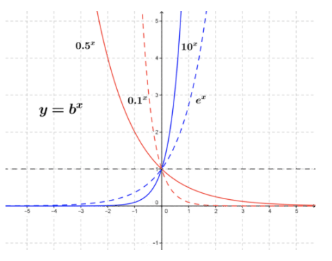
The figure below shows a few exponential function graphs for 0<b≤10. It is very clear that the sign of the derivative of an exponential depends on the value of b. If 0<b<1, the value of the derivative of the function (slope of the tangent line) will be negative because the function is always decreasing as x increases. For b>1, the derivative of the function will always be positive because the function increases as x increases.

CC BY-NC-SA
But, what is the derivative of an exponential function? We can take the following steps to find an expression for \( \dfrac{d}{dx}[bx] \nonumber\) by using the definition of the derivative:
\( \displaystyle \dfrac{d}{dx}[bx]= \lim_{h \to 0} \dfrac{b^{x+h}−b^x}{h} \nonumber\).... Limit definition of the derivative
\( = \lim_{h \to 0} \dfrac{b^xb^h−b^x}{h} \nonumber\)....Exponent property
\( = \lim_{h \to 0} \dfrac{b^h−1}{h}⋅b^x \nonumber\)....Factoring
\( = ( \lim_{h→0} \dfrac{b^h−1}{h})⋅bx \nonumber\)....Limit of a product property
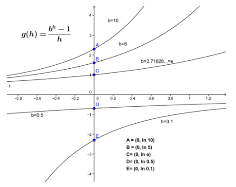
The result above shows \( \dfrac{d}{dx}[bx] \nonumber\) depends on the product of \( \lim_{h→0} \dfrac{b^h−1}{h} \nonumber\) and the original function. But what is \( \lim_{h→0} \dfrac{b^h−1}{h} \nonumber\)? There are a number of ways to evaluate this limit, but for now let’s take a quick look at the behavior of \( \dfrac{b^h−1}{h} \nonumber\). This function is graphed below for a number of values of b, and the limit at \( h=0 \nonumber\) is indicated by the points A−E.

CC BY-NC-SA
While it is not at all obvious:\( \lim_{h→0} \dfrac{b^h−1}{h} = ln(b) \nonumber\). Remember the natural logarithm function \( y=lnx \nonumber\) on your calculator? The natural logarithm is the general logarithm function with base \( b=e=2.71828 \nonumber\)...
Given the exponential function \( f(x)=b^x \nonumber\), where the base b is a positive, real number, then the general representation of the derivative of an exponential function is:
\[ \dfrac{d}{dx}[bx]=lnb⋅b^x \nonumber\]
Adding the Chain Rule to the definition, given the exponential function f(x)=bu, where u=g(x) and g(x) is a differentiable function, then:
\[ \dfrac{d}{dx}[bu]=(lnb⋅b^u) \dfrac{du}{dx} \nonumber\]
Examples
Example 1
Earlier, you were asked what the general exponential equation for the growth of a population that doubles every 5 years is.
A population \( P(t) \nonumber\) that doubles every 5 years could be modeled as \( P(t)=P_02^{\dfrac{t}{5}} \nonumber\), where the variable t represents number of years since the population was at a level of \( P_0 \nonumber] \nonumber\). Were you able to determine that the rate of change of \( P(t) \nonumber\) is \( P′(t) = \dfrac{P_0 ln2}{5}⋅2^{\dfrac{t}{5}} \nonumber\)?
Example 2
Given \( y=500⋅0.7^x \nonumber\), what is \( \dfrac{dy}{dx} \nonumber\)?
\[ \dfrac{dy}{dx}=\dfrac{d}{dx}[500⋅0.7^x] \nonumber\]
\[ = 500 \dfrac{d}{dx}[0.7^x] \nonumber\]
\( = 500[ln(0.7)⋅0.7^x] \nonumber\)....Use your calculator to find ln(0.7)
\[ =−178.3⋅0.7^x \nonumber\]
Hence, \( \dfrac{dy}{dx} =−178.3⋅0.7^x \nonumber\), and as expected, the slopes of all tangent lines are negative.
There is an important special case that you must know about
Example 3
Given \( y=500⋅e^x \nonumber\), what is \( \dfrac{dy}{dx} \nonumber\)?
\[ \dfrac{dy}{dx}= \dfrac{d}{dx}[500⋅ex] \nonumber\]
\[ = 500 \dfrac{d}{dx}[ex] \nonumber\]
\( \dfrac{dy}{dx}=500[ln(e)⋅ex] \nonumber\)....Use your calculator to find ln(e)
\[ = \dfrac{d}{dx}[500⋅ex] \nonumber\]
\[ =500[1⋅ex] \nonumber\]
\[ =500⋅ex \nonumber\]
Hence, \( \dfrac{dy}{dx}=500⋅ex \nonumber\), and this is just the original function. This exponential function, with base e, is special: the rate of change (or slope of the tanget line) at any point is equal to the value of the function at that point.
Example 4
Given \( y=10⋅2.5−3x^2 \nonumber\), what is \( \dfrac{dy}{dx} \nonumber\)?
\[ \dfrac{dy}{dx} = \dfrac{d}{dx}[10⋅2.5−3x2] \nonumber\]
\[ =10 \dfrac{d}{dx}[2.5−3x2] \nonumber\]
\[ =10⋅ln(2.5)⋅2.5−3x2⋅ddx[−3x^2] \nonumber\]
\[ =10⋅(0.9162)⋅2.5−3x^2⋅[−6x] \nonumber\]
\[ =−55x⋅2.5−3x^2 \nonumber\]
Therefore, \( \dfrac{dy}{dx} =−55x⋅2.5−3x^2 \nonumber\)
Example 5
Given \( y=500⋅e−2x⋅cos(5πx) \nonumber\), what is \( \dfrac{dy}{dx} \nonumber\)?
\[ \dfrac{dy}{dx}= \dfrac{d}{dx}[500⋅e−2x⋅cos(5πx)] \nonumber\]
\( =500⋅[ \dfrac{d}{dx}(e−2x)⋅cos(5πx)+e−2x⋅ \dfrac{d}{dx}(cos(5πx))] \nonumber\)....Product Rule
\( =500⋅[ln(e)⋅e−2x \dfrac{d}{dx}(−2x)⋅cos(5πx)+e−2x⋅(−sin(5πx)⋅ \dfrac{d}{dx}(5πx))] \nonumber\)....Use Chain Rule
\( =500⋅[(1)⋅e−2x⋅(−2)⋅cos(5πx)+e−2x⋅(−sin(5πx)⋅5π)] \nonumber\)....Simplify.
\( =−500⋅e−2x[2⋅cos(5πx)+5πsin(5πx)] \nonumber\)...Simplify
Therefore, \( \dfrac{dy}{dx} =−500⋅e−2x[2⋅cos(5πx)+5πsin(5πx)] \nonumber\).
Review
For #1-14, find the derivative.
- \( y=7^x \nonumber\)
- \( y=3^{2x} \nonumber\)
- \( y=5^x−3x^2 \nonumber\)
- \( y=2^{x^2} \nonumber\)
- \( y=e^{x^2} \nonumber\)
- \(f(x)= \dfrac{1}{ \sqrt{πσ}}e^{−αk(x−x0)^2} \nonumber\) where σ, α, x0, and k are constants and σ≠0.
- \( y=e^{6x} \nonumber\)
- \( y=e^{3x^3}−2x^2+6 \nonumber\)
- \( y=\dfrac{e^x−e−x}{e^x+e−x} \nonumber\)
- \( y=cos(e^x) \nonumber\)
- \( y=e^{−x}3^x \nonumber\)
- \( y=3^{−x^2+2x+1} \nonumber\)
- \( y=2^x3^x \nonumber\)
- \( y=e^{−x}sinx \nonumber\)
- Find an equation of the tangent line to \( f(x)=x^3+2e^x \nonumber\) at the point (0, 2).
Vocabulary
| Term | Definition |
|---|---|
| derivative | The derivative of a function is the slope of the line tangent to the function at a given point on the graph. Notations for derivative include f′(x), dydx, y′, dfdx and \dfrac{df(x)}{dx}. |
| Exponential Function | An exponential function is a function whose variable is in the exponent. The general form is \( y=a⋅b^{x−h}+k \nonumber\). |

