7.2: Absolute versus Local Extrema
- Page ID
- 1214
\( \newcommand{\vecs}[1]{\overset { \scriptstyle \rightharpoonup} {\mathbf{#1}} } \)
\( \newcommand{\vecd}[1]{\overset{-\!-\!\rightharpoonup}{\vphantom{a}\smash {#1}}} \)
\( \newcommand{\id}{\mathrm{id}}\) \( \newcommand{\Span}{\mathrm{span}}\)
( \newcommand{\kernel}{\mathrm{null}\,}\) \( \newcommand{\range}{\mathrm{range}\,}\)
\( \newcommand{\RealPart}{\mathrm{Re}}\) \( \newcommand{\ImaginaryPart}{\mathrm{Im}}\)
\( \newcommand{\Argument}{\mathrm{Arg}}\) \( \newcommand{\norm}[1]{\| #1 \|}\)
\( \newcommand{\inner}[2]{\langle #1, #2 \rangle}\)
\( \newcommand{\Span}{\mathrm{span}}\)
\( \newcommand{\id}{\mathrm{id}}\)
\( \newcommand{\Span}{\mathrm{span}}\)
\( \newcommand{\kernel}{\mathrm{null}\,}\)
\( \newcommand{\range}{\mathrm{range}\,}\)
\( \newcommand{\RealPart}{\mathrm{Re}}\)
\( \newcommand{\ImaginaryPart}{\mathrm{Im}}\)
\( \newcommand{\Argument}{\mathrm{Arg}}\)
\( \newcommand{\norm}[1]{\| #1 \|}\)
\( \newcommand{\inner}[2]{\langle #1, #2 \rangle}\)
\( \newcommand{\Span}{\mathrm{span}}\) \( \newcommand{\AA}{\unicode[.8,0]{x212B}}\)
\( \newcommand{\vectorA}[1]{\vec{#1}} % arrow\)
\( \newcommand{\vectorAt}[1]{\vec{\text{#1}}} % arrow\)
\( \newcommand{\vectorB}[1]{\overset { \scriptstyle \rightharpoonup} {\mathbf{#1}} } \)
\( \newcommand{\vectorC}[1]{\textbf{#1}} \)
\( \newcommand{\vectorD}[1]{\overrightarrow{#1}} \)
\( \newcommand{\vectorDt}[1]{\overrightarrow{\text{#1}}} \)
\( \newcommand{\vectE}[1]{\overset{-\!-\!\rightharpoonup}{\vphantom{a}\smash{\mathbf {#1}}}} \)
\( \newcommand{\vecs}[1]{\overset { \scriptstyle \rightharpoonup} {\mathbf{#1}} } \)
\( \newcommand{\vecd}[1]{\overset{-\!-\!\rightharpoonup}{\vphantom{a}\smash {#1}}} \)
\(\newcommand{\avec}{\mathbf a}\) \(\newcommand{\bvec}{\mathbf b}\) \(\newcommand{\cvec}{\mathbf c}\) \(\newcommand{\dvec}{\mathbf d}\) \(\newcommand{\dtil}{\widetilde{\mathbf d}}\) \(\newcommand{\evec}{\mathbf e}\) \(\newcommand{\fvec}{\mathbf f}\) \(\newcommand{\nvec}{\mathbf n}\) \(\newcommand{\pvec}{\mathbf p}\) \(\newcommand{\qvec}{\mathbf q}\) \(\newcommand{\svec}{\mathbf s}\) \(\newcommand{\tvec}{\mathbf t}\) \(\newcommand{\uvec}{\mathbf u}\) \(\newcommand{\vvec}{\mathbf v}\) \(\newcommand{\wvec}{\mathbf w}\) \(\newcommand{\xvec}{\mathbf x}\) \(\newcommand{\yvec}{\mathbf y}\) \(\newcommand{\zvec}{\mathbf z}\) \(\newcommand{\rvec}{\mathbf r}\) \(\newcommand{\mvec}{\mathbf m}\) \(\newcommand{\zerovec}{\mathbf 0}\) \(\newcommand{\onevec}{\mathbf 1}\) \(\newcommand{\real}{\mathbb R}\) \(\newcommand{\twovec}[2]{\left[\begin{array}{r}#1 \\ #2 \end{array}\right]}\) \(\newcommand{\ctwovec}[2]{\left[\begin{array}{c}#1 \\ #2 \end{array}\right]}\) \(\newcommand{\threevec}[3]{\left[\begin{array}{r}#1 \\ #2 \\ #3 \end{array}\right]}\) \(\newcommand{\cthreevec}[3]{\left[\begin{array}{c}#1 \\ #2 \\ #3 \end{array}\right]}\) \(\newcommand{\fourvec}[4]{\left[\begin{array}{r}#1 \\ #2 \\ #3 \\ #4 \end{array}\right]}\) \(\newcommand{\cfourvec}[4]{\left[\begin{array}{c}#1 \\ #2 \\ #3 \\ #4 \end{array}\right]}\) \(\newcommand{\fivevec}[5]{\left[\begin{array}{r}#1 \\ #2 \\ #3 \\ #4 \\ #5 \\ \end{array}\right]}\) \(\newcommand{\cfivevec}[5]{\left[\begin{array}{c}#1 \\ #2 \\ #3 \\ #4 \\ #5 \\ \end{array}\right]}\) \(\newcommand{\mattwo}[4]{\left[\begin{array}{rr}#1 \amp #2 \\ #3 \amp #4 \\ \end{array}\right]}\) \(\newcommand{\laspan}[1]{\text{Span}\{#1\}}\) \(\newcommand{\bcal}{\cal B}\) \(\newcommand{\ccal}{\cal C}\) \(\newcommand{\scal}{\cal S}\) \(\newcommand{\wcal}{\cal W}\) \(\newcommand{\ecal}{\cal E}\) \(\newcommand{\coords}[2]{\left\{#1\right\}_{#2}}\) \(\newcommand{\gray}[1]{\color{gray}{#1}}\) \(\newcommand{\lgray}[1]{\color{lightgray}{#1}}\) \(\newcommand{\rank}{\operatorname{rank}}\) \(\newcommand{\row}{\text{Row}}\) \(\newcommand{\col}{\text{Col}}\) \(\renewcommand{\row}{\text{Row}}\) \(\newcommand{\nul}{\text{Nul}}\) \(\newcommand{\var}{\text{Var}}\) \(\newcommand{\corr}{\text{corr}}\) \(\newcommand{\len}[1]{\left|#1\right|}\) \(\newcommand{\bbar}{\overline{\bvec}}\) \(\newcommand{\bhat}{\widehat{\bvec}}\) \(\newcommand{\bperp}{\bvec^\perp}\) \(\newcommand{\xhat}{\widehat{\xvec}}\) \(\newcommand{\vhat}{\widehat{\vvec}}\) \(\newcommand{\uhat}{\widehat{\uvec}}\) \(\newcommand{\what}{\widehat{\wvec}}\) \(\newcommand{\Sighat}{\widehat{\Sigma}}\) \(\newcommand{\lt}{<}\) \(\newcommand{\gt}{>}\) \(\newcommand{\amp}{&}\) \(\definecolor{fillinmathshade}{gray}{0.9}\)Being able to identify the smallest and largest values of a function (extrema), and where they occur in some interval on the domain or over the entire domain, is useful in graphing a function equation as well as in solving “optimization” problems. The location of these extrema is tied to the behavior of the derivative. You learned in prior work with quadratic functions (parabolas, \( y=ax^2+bx+c \nonumber\)), that the least or greatest value of the parabola could be found at the vertex of the parabola (on the axis of symmetry \( x=− \frac{b}{2a} \nonumber\)). How are the derivative of the quadratic function and the vertex \( x=− \frac{b}{2a} \nonumber\) related?
Extrema
Let’s start our discussion with some formal working definitions of the maximum and minimum values of a function.
- A function f has a maximum at x=a if \( f(a)≥f(x) \nonumber\) for all x in the domain of f.
- A function f has a minimum at x=a if \( f(a)≤f(x) \nonumber\) for all x in the domain of f.
The values of the function for these x-values are called extreme values or extrema.
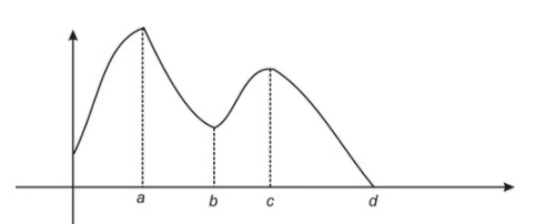
Here is an example of a function that has a maximum at x=a and a minimum at x=d:
CC BY-NC-SA
Observe the graph at x=b. While we do not have a minimum at x=b, we note that f(b)≤f(x) for all x near b. We say that the function has a local minimum at x=b.
Similarly, we say that the function has a local maximum at x=c since f(c)≥f(x) for some x contained in open intervals of c.
Remember to use the terms maximum and minimum (without including the term local) only when you are talking about the absolute or global extrema values of the function; local extrema or relative extrema should be called local maximum or local minimum.
Do all functions have a maximum and minimum? Yes, all continuous functions do. This is stated by the Extreme Value Theorem that we discussed in the concept on Continuity.
Extreme Value Theorem: If a function f(x) is continuous in a closed interval I, then f(x) has both a maximum value and a minimum value in I.
This makes sense conceptually. Try drawing a function (on a closed interval, including the endpoints) so that no point is at the highest part of the graph. No matter how the function is sketched, there will be at least one point that is highest.
How do extreme values, maxima and minima, relate to derivatives? The French mathematician Fermat shows how in Fermat's Theorem: If f(c) is an extreme value of f for some open interval containing c, then either f′(c)=0, or f′(c) does not exist.
This relationship between the location of extrema and the derivative at the location is so important that we give the location the name critical point.
We will call x=c a critical point in the closed interval [a,b] if f(c) exists, and either f′(c)=0 or f′(c) does not exist.
Summary so far: If a function is continuous in a closed interval, it has both a minimum and a maximum at some location(s), and the derivative at these locations is either 0 or does not exist. The locations are called critical points.
The diagram below explicitly identifies how to identify critical points. The end points of the closed interval are included as critical points if we consider the function only defined on the closed interval and not outside the interval. In this case, the derivative at each end point would not be defined.
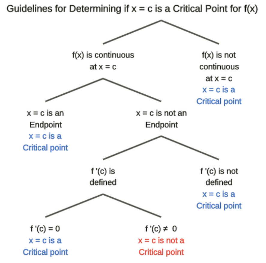
A tree diagram to help identify critical points. CK-12 Foundation
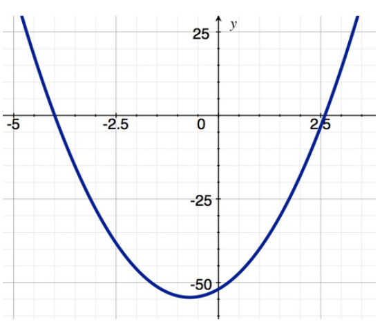
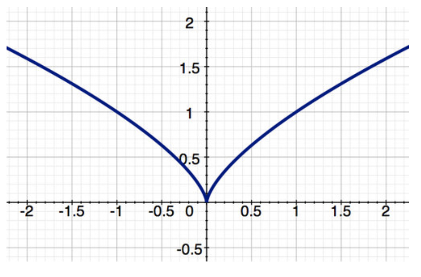
Let’s consider the two functions shown below and say something about them in the closed interval [-2, 2]. Notice that g(x) (the second function) has a cusp at x=0.
Two functions
Both functions are continuous in [-2, 2]. By the Extreme Value Theorem they both have a minimum and maximum. As the table shows, f(x) has an extreme value where f′(x)=0, and g(x) has an extreme value where g′(x) is not defined. These are critical points.
| Function Property | \( f(x)=5x^2+7x−52 \nonumber\) | \( g(x)=x^{\frac{2}{3}} \nonumber\) |
| Value at endpoint x=−2 | -46 | 1.59 |
| Value at endpoint x=2 | -18 | 1.59 |
| Location and value where f′(x)=0 | (-0.7, -54.45) | --- |
| Location where f′(x) Does Not Exist | End points | Endpoints, x=0 |
| Critical point(s) | x=−0.7 End points | x=0, End points |
| Minimum value and location(s) | (-0.7, -54.45) | (0, 0) |
| Location(s) of Maximum value | (2, -18) | (-2, 1.59) (2, 1.59) |
It should be noted that the converse of the Extreme Value Theorem is not necessarily true, i.e., just because f′(x)=0 at some location x=a, the function value f(a) does not have to be a local minimum or maximum.
Consider \( f(x)=x^3 \nonumber\) and its graph. We see that while f′(0)=0 at x=0, x=0 is not an extreme point of the function.
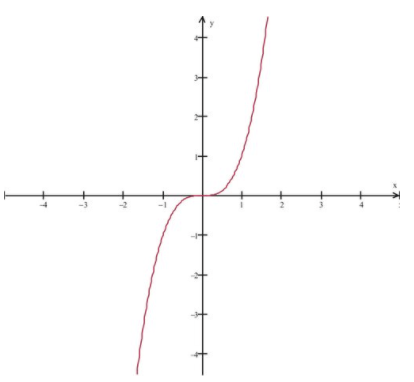
CC BY-NC-SA
Examples
Example 1
Earlier, you were asked to determine how the derivative of the quadratic function \( (y=ax^2+bx+c) \nonumber\) and the vertex formula \( x=− \frac{b}{2a} \nonumber\) are related.
If you realized that the vertex of the quadratic function is also the location where the slope of the tangent line, and therefore the derivative, equals 0 you made a great observation. \( \frac{dy}{dx}=2ax+b=0 \nonumber\) means that \( x=− \frac{b}{2a} \nonumber\). This is the x-value of the vertex, and a critical value or point of the function.
Example 2
The function \( f(x)= \sqrt{25−x^2} \nonumber\) is the upper portion of a circle centered at (0, 0) with radius 5. Find the critical points of the function, and the maxima and minima.
Compute the derivative: \( f′(x) = \frac{1}{2 \sqrt{25−x^2}}(−2x) = − \frac{x}{ \sqrt{25−x^2}} \nonumber\)
f′(x)=0 means x=0 is a critical point, and f(0)=5.
Notice that f′(x) is undefined at the two locations x=±5, which means these are critical points. Both of the values are associated with function values f(±5)=0.
The function minima are at (-5, 0) and (5, 0); the function maximum is at (0, 5).
Review
For #1-3, identify the absolute and local minimum and maximum values of the function (if they exist); find the extrema. (Units on the axes indicate1 unit).
- Continuous on [0, 9]
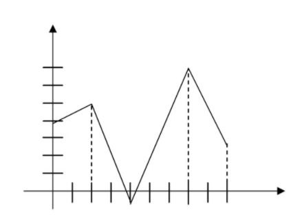
CC BY-NC-SA
- Continuous on [0, 9]
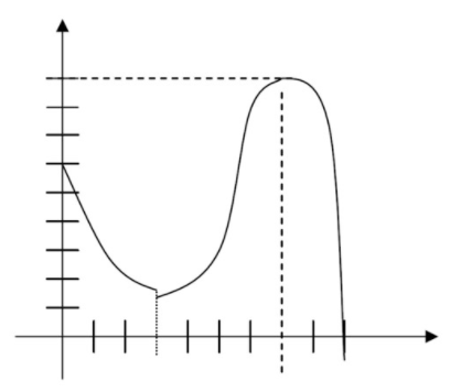
CC BY-NC-SA
- Continuous on [0,4]∪[4,9]
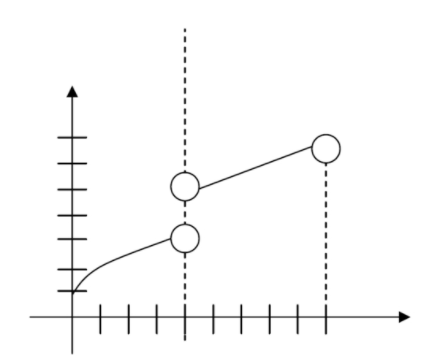
CC BY-NC-SA
For #4–6, find the extrema and sketch the graph.
- \( f(x)=−x^2−6x+4, [-4, 1] \nonumber\)
- \( f(x)=x^3−x^4, [0, 2] \nonumber\)
- \( f(x)=−x^2+4x^2, [-2, 0] \nonumber\)
- What is the absolute maximum of the sine function over the interval \( [0,π] \nonumber\)?
- What are the local minimums of the cosine function over the interval \( [0,2π] \nonumber\)?
- What is the absolute maximum and absolute minimum of the function \( x^2 \nonumber\) over the interval [6, 7]?
- At what point does the function \( f(x)=(x^2−7x−8)^4 \nonumber\) attain its absolute minimum over the interval [5, 10]?
- Let [a,b] be a closed, finite interval, and let f(x) be a straight line. If f(x) achieves its maximum value over [a,b] at points other than a and b, what must be true about f(x)?
- Find all the critical numbers of \( f(x)=3x^4− \frac{8}{3}x^3−6x^2+8x+1 \nonumber\).
- Find all the critical numbers of \( f(x)=\frac{1}{2x^2−5x−3} \nonumber\).
- Find all the critical numbers of \( f(x)=ln(x−4) \nonumber\).
- Find all the critical numbers of \( f(x)=\sqrt{x} ×(1−x) \nonumber\).
- Find all the critical numbers of \( f(x)= \frac{x^2+x+1}{x−2} \nonumber\).
- Does the polynomial \( f(x)=x^6+x^4+x^2+1 \nonumber\) attain a minimum value over the interval \( [−π,π] \nonumber\)?
- Does the function \( f(x)=7^{sin(x)} \nonumber\) attain a maximum value over the interval \( (0,π) ] \nonumber\)?
- Does the function \( f(x)= \frac{10}{x} \nonumber\) attain a maximum value over the interval [-1, 1]?
- Does the function \( f(x)=sin( \frac{x}{2}) \nonumber\) attain a minimum value over the interval \( (0,π) \nonumber\)?
- Let a and b be two positive number such that a<b. Does the function f(x)=ln(x) attain a maximum value over the interval [a,b]?
Vocabulary
| Term | Definition |
|---|---|
| critical point | A critical value (or point) is a value in a closed interval of the domain of the function where either the function derivative at the point is 0, or the derivative does not exist. |
| derivative | The derivative of a function is the slope of the line tangent to the function at a given point on the graph. Notations for derivative include f′(x), \( \frac{dy}{dx} \nonumber\), y′, \( \frac{df}{dx} \nonumber\) and \frac{df(x)}{dx}. |
| Extrema | Extrema is a collective term encompassing both the minimum and maximum values, referring to the "extreme" values of the function. |
| global extrema | The global extrema of a function are the points with the y values that are the highest or the lowest of the entire function. |
| Global Maximum | The global maximum of a function is the largest value of the entire function. Symbolically, it is the highest point on the entire graph. |
| Global Minimum | The global minimum of a function is the smallest value of the entire function. Symbolically, it is the lowest point on the entire graph. |
| local extrema | The local extrema of a function are the points of the function with y values that are the highest or lowest of a local neighborhood of the function. |
| Local Maximum | A local maximum is the highest point relative to the points around it. A function can have more than one local maximum. |
| Local Minimum | A local minimum is the lowest point relative to the points around it. A function can have more than one local minimum. |
| Maximum | The maximum is the highest point of a graph. The maximum will yield the largest value of the range. |
| Minimum | The minimum is the lowest point of a graph. The minimum will yield the smallest value of the range. |
Additional Resources
PLIX: Play, Learn, Interact, eXplore - Absolute versus Local Extrema
Video: Local and Absolute Maximum and Minimum
Practice: Absolute versus Local Extrema

