7.3: First Derivative Test

If you look at any function curve, you can determine visually whether the function is increasing, decreasing, or remaining constant over an interval. You can also see approximately were the function attains high points and low points. There is a way to determine mathematically, using the derivative, what your visual observations provide. How does knowing the slope of a tangent line help you to precisely calculate what your visual observations can only estimate?

---

The First Derivative Test

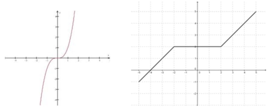
Consider the graphs of the two functions below.

CC BY-NC-SA

Both functions are continuous over the intervals shown. In the first, \( f(x)=x^3 \nonumber\), the function values are always increasing as x increases. In the second, the piece-wise function values increase over the interval [-5, -2], stay the same over the interval [-2, 2], then resume increasing for [2, 5].

The difference between these two cases of increasing function values motivates the need for the following distinctions:

• A function f is said to be increasing on [a,b] contained in the domain of f if \( f(x_1)≤f(x_2) \nonumber\) whenever \( x_1≤x_2 \nonumber\)  for all \( x_1,x_2∈[a,b] \nonumber\).
• If \( f(x_1)<f(x_2) \nonumber\) whenever \( x_1<x_2 \nonumber\) for all \( x_1,x_2∈[a,b] \nonumber\), then we say that f is strictly increasing on  [a,b].

In similar manner:

• A function f is said to be decreasing on [a,b] contained in the domain of f if \( f(x_1)≤f(x_2) \nonumber\) whenever \( x_1≥x_2 \nonumber\) for all \( x_1,x_2∈[a,b] \nonumber\).
• If \( f(x_1)>f(x_2) \nonumber\) whenever \( x_1>x_2 \nonumber\) for all \( x_1,x_2∈[a,b] \nonumber\). Then we say that f is strictly decreasing on [a,b].

Note that the symbols \( ϵ \nonumber\) and \( ∈ \nonumber\) are equivalent and denote that a particular element is contained within a particular set.

Using the above terminology, we say the function \( f(x)=x^3 \nonumber\) is strictly increasing over the given interval, and the piece-wise function is increasing over the interval.

Now look at the derivatives of the two functions graphed above.

We can now state a theorem that relates the derivative of a function to the increasing/decreasing properties of the function.

If f is continuous on interval [a,b], and differentiable on (a,b) then:

• If f′(x)>0 for every \( x∈(a,b) \nonumber\), then f is increasing in [a,b].
• If f′(x)<0 for every\( x∈(a,b) \nonumber\), then f is decreasing in [a,b].

Take the function \( f(x)=x^3−3x^2−6x+8 \nonumber\). To find the intervals on which f is increasing and the intervals on which f is decreasing, first note that the function f(x) is continuous everywhere. The derivative of the function is \( f′(x)=3x^2−6x−6=3(x^2−2x−2) \nonumber\), which is a parabola with two x-intercepts (critical numbers of f) at \( x=1±\sqrt{3} \nonumber\). Evaluation of f′(x) in the three intervals that are defined by the two roots provides the following information:

\[ f'(x) = \begin{cases} >0, & x<1- \sqrt{3} & f(x) \mbox{ is increasing} \\ =0, & x = 1 - \sqrt{3} \\ <0 & (1- \sqrt{3})<x<(1+ \sqrt{3}) & f(x) \mbox{ is decreasing} \\ =0, & x = 1 + \sqrt{3} \\ >0, & x>1+ \sqrt{3} & f(x) \mbox{ is increasing} \end{cases} \nonumber\]

Changes in the derivative of a function from positive to negative, or negative to positive may indicate the presence of a local extremum.

The First Derivative Test describes where these extrema are and what type they are. The First Derivative Test is as follows:

Suppose that f is a continuous function and that x=c is a critical value of f, then:

1. If f′ changes from positive to negative at x=c, then f has a local maximum at x=c.
2. If f′ changes from negative to positive at x=c, then f has a local minimum at x=c.
3. If f′ does not change sign at x=c, then f has neither a local maximum nor minimum at x=c.

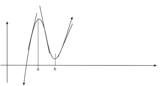
We can observe the consequences of this theorem by observing the tangent lines of the following graph in each of the intervals (0,a), (a,b), (b,+∞).

CC BY-NC-SA

Note first that we have a relative maximum at x=a and a relative minimum at x=b. The slopes of the tangent lines change from positive for x∈(0,a) to negative for x∈(a,b) and then back to positive for x∈(b,+∞).

---

Examples

Example 1

Earlier, you were asked how the slope of the tangent line relates to whether or not a function is increasing or decreasing. Positive slope means an increasing function; negative slope means a decreasing function. Often the slope transition from positive (negative) to negative (positive) indicates the location of an extremum.

Example 2

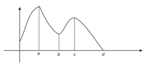
Consider the function graph below. Determine whether the function where the function is strictly increasing or decreasing.

CC BY-NC-SA

The function indicated here is strictly increasing on (0,a) and (b,c), and strictly decreasing on (a,b) and (c,d).

Example 3

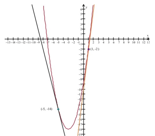
Let's consider the function \( f(x)=x^2+6x−9 \nonumber\) and observe the graph around x=−3. What happens to the first derivative near this value?

CC BY-NC-SA

With \( f(x)=x^2+6x−9 \nonumber\), the derivative is \( f′(x)=2x+6 \nonumber\). Notice that the following condition applies to the slopes of tangent lines:

\[ f'(x) \begin{cases} <0, & x < -3 \\ =0, & x = 0 \\ >0, & x > -3 \end{cases} \nonumber\]

We observe that the slopes of the tangent lines to the graph change from negative to positive at x=−3. The first derivative test states that f(x) has a local minimum at x=−3. The function graph verifies this.

---

Review

For #1-2, identify the intervals where the function is increasing, decreasing, or is constant. (Units on the axes indicate single units).

1. 

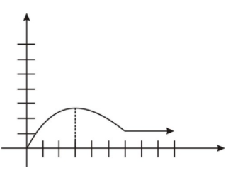
figure5

2. 

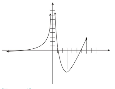
figure6

3. Give the sign of the following quantities for the graph in problem 2.

1. f′(−3)
2. f′(1)
3. f′(3)
4. f′(4)

For #4-6, determine the intervals in which the function is increasing and those in which it is decreasing, then sketch the graph of each function.

4. \( f(x)=x^2−\frac{1}{x} \nonumber\) 
5. \( f(x)= (x^2−1)^5 \nonumber\)
6. \( f(x)=(x^2−1)^4 \nonumber\)

For #7-10:

• Use the First Derivative Test to find the intervals where the function increases and/or decreases
• Identify all max, min, or relative max and min values
• Sketch the graph

7. \( f(x)=−x^2−4x−1 \nonumber\)
8. \( f(x)=x^3+3x^2−9x+1 \nonumber\)
9. \( f(x)=x^{ \frac{2}{3}}(x−5) \nonumber\)
10. \( f(x)=2x \sqrt{x2+1} \nonumber\)
11. Use the first derivative test to classify the critical numbers \( x=0 \nonumber\) and \( x= \frac{3π}{2} \nonumber\) of \( f(x)=cos^2(x) \nonumber\) as local maxima or minima.
12. Find the critical numbers of \( f(x)=x^5−20x−2 \nonumber\) and classify them as local maxima, minima or neither.
13. Find the local extrema of \( f(x)=x+sin(x) \nonumber\) on the interval \( (−2π,2π) \nonumber\).
14. Find the global and local extrema of \( f(x)=\frac{3}{4}x^4+4x^3−6x^2−48x−50 \nonumber\).
15. Find the global and local extrema of \( f(x)= \frac{x^2−x−6}{x^2+x−6} \nonumber\).

---

Review (Answers)

To see the Review answers, open this PDF file and look for section 4.4. 

---

Vocabulary

Term	Definition
decreasing function	A decreasing function is one with a graph that goes down from left to right.
first derivative test	The first derivative test says that if f is a continuous function and that x=c is a critical value of f, then if f′ changes from positive to negative at x=c then f has a local maximum at x=c, if f′ changes from negative to positive at x=c then f has a local minimum at x=c, and if f′ does not change sign at x=c then f has neither a local maximum nor minimum at x=c.
increasing function	An increasing function is one with a graph that goes up from left to right.
strictly	Strictly is an adjective that alters increasing and decreasing to exclude any flatness or periods where y values are staying constant.

---

Additional Resources

Video: Identifying Minima and Maxima

Real World: Losing Ground