8.1: Absolute Extrema and Optimization

Last updated
Save as PDF

Page ID: 1203

$ \newcommand{\vecs}[1]{\overset { \scriptstyle \rightharpoonup} {\mathbf{#1}} } $

$ \newcommand{\vecd}[1]{\overset{-\!-\!\rightharpoonup}{\vphantom{a}\smash {#1}}} $

$ \newcommand{\id}{\mathrm{id}}$ $ \newcommand{\Span}{\mathrm{span}}$

( \newcommand{\kernel}{\mathrm{null}\,}\) $ \newcommand{\range}{\mathrm{range}\,}$

$ \newcommand{\RealPart}{\mathrm{Re}}$ $ \newcommand{\ImaginaryPart}{\mathrm{Im}}$

$ \newcommand{\Argument}{\mathrm{Arg}}$ $ \newcommand{\norm}[1]{\| #1 \|}$

$ \newcommand{\inner}[2]{\langle #1, #2 \rangle}$

$ \newcommand{\Span}{\mathrm{span}}$

$ \newcommand{\id}{\mathrm{id}}$

$ \newcommand{\Span}{\mathrm{span}}$

$ \newcommand{\kernel}{\mathrm{null}\,}$

$ \newcommand{\range}{\mathrm{range}\,}$

$ \newcommand{\RealPart}{\mathrm{Re}}$

$ \newcommand{\ImaginaryPart}{\mathrm{Im}}$

$ \newcommand{\Argument}{\mathrm{Arg}}$

$ \newcommand{\norm}[1]{\| #1 \|}$

$ \newcommand{\inner}[2]{\langle #1, #2 \rangle}$

$ \newcommand{\Span}{\mathrm{span}}$ $ \newcommand{\AA}{\unicode[.8,0]{x212B}}$

$ \newcommand{\vectorA}[1]{\vec{#1}} % arrow$

$ \newcommand{\vectorAt}[1]{\vec{\text{#1}}} % arrow$

$ \newcommand{\vectorB}[1]{\overset { \scriptstyle \rightharpoonup} {\mathbf{#1}} } $

$ \newcommand{\vectorC}[1]{\textbf{#1}} $

$ \newcommand{\vectorD}[1]{\overrightarrow{#1}} $

$ \newcommand{\vectorDt}[1]{\overrightarrow{\text{#1}}} $

$ \newcommand{\vectE}[1]{\overset{-\!-\!\rightharpoonup}{\vphantom{a}\smash{\mathbf {#1}}}} $

$ \newcommand{\vecs}[1]{\overset { \scriptstyle \rightharpoonup} {\mathbf{#1}} } $

$ \newcommand{\vecd}[1]{\overset{-\!-\!\rightharpoonup}{\vphantom{a}\smash {#1}}} $

$\newcommand{\avec}{\mathbf a}$ $\newcommand{\bvec}{\mathbf b}$ $\newcommand{\cvec}{\mathbf c}$ $\newcommand{\dvec}{\mathbf d}$ $\newcommand{\dtil}{\widetilde{\mathbf d}}$ $\newcommand{\evec}{\mathbf e}$ $\newcommand{\fvec}{\mathbf f}$ $\newcommand{\nvec}{\mathbf n}$ $\newcommand{\pvec}{\mathbf p}$ $\newcommand{\qvec}{\mathbf q}$ $\newcommand{\svec}{\mathbf s}$ $\newcommand{\tvec}{\mathbf t}$ $\newcommand{\uvec}{\mathbf u}$ $\newcommand{\vvec}{\mathbf v}$ $\newcommand{\wvec}{\mathbf w}$ $\newcommand{\xvec}{\mathbf x}$ $\newcommand{\yvec}{\mathbf y}$ $\newcommand{\zvec}{\mathbf z}$ $\newcommand{\rvec}{\mathbf r}$ $\newcommand{\mvec}{\mathbf m}$ $\newcommand{\zerovec}{\mathbf 0}$ $\newcommand{\onevec}{\mathbf 1}$ $\newcommand{\real}{\mathbb R}$ $\newcommand{\twovec}[2]{\left[\begin{array}{r}#1 \\ #2 \end{array}\right]}$ $\newcommand{\ctwovec}[2]{\left[\begin{array}{c}#1 \\ #2 \end{array}\right]}$ $\newcommand{\threevec}[3]{\left[\begin{array}{r}#1 \\ #2 \\ #3 \end{array}\right]}$ $\newcommand{\cthreevec}[3]{\left[\begin{array}{c}#1 \\ #2 \\ #3 \end{array}\right]}$ $\newcommand{\fourvec}[4]{\left[\begin{array}{r}#1 \\ #2 \\ #3 \\ #4 \end{array}\right]}$ $\newcommand{\cfourvec}[4]{\left[\begin{array}{c}#1 \\ #2 \\ #3 \\ #4 \end{array}\right]}$ $\newcommand{\fivevec}[5]{\left[\begin{array}{r}#1 \\ #2 \\ #3 \\ #4 \\ #5 \\ \end{array}\right]}$ $\newcommand{\cfivevec}[5]{\left[\begin{array}{c}#1 \\ #2 \\ #3 \\ #4 \\ #5 \\ \end{array}\right]}$ $\newcommand{\mattwo}[4]{\left[\begin{array}{rr}#1 \amp #2 \\ #3 \amp #4 \\ \end{array}\right]}$ $\newcommand{\laspan}[1]{\text{Span}\{#1\}}$ $\newcommand{\bcal}{\cal B}$ $\newcommand{\ccal}{\cal C}$ $\newcommand{\scal}{\cal S}$ $\newcommand{\wcal}{\cal W}$ $\newcommand{\ecal}{\cal E}$ $\newcommand{\coords}[2]{\left\{#1\right\}_{#2}}$ $\newcommand{\gray}[1]{\color{gray}{#1}}$ $\newcommand{\lgray}[1]{\color{lightgray}{#1}}$ $\newcommand{\rank}{\operatorname{rank}}$ $\newcommand{\row}{\text{Row}}$ $\newcommand{\col}{\text{Col}}$ $\renewcommand{\row}{\text{Row}}$ $\newcommand{\nul}{\text{Nul}}$ $\newcommand{\var}{\text{Var}}$ $\newcommand{\corr}{\text{corr}}$ $\newcommand{\len}[1]{\left|#1\right|}$ $\newcommand{\bbar}{\overline{\bvec}}$ $\newcommand{\bhat}{\widehat{\bvec}}$ $\newcommand{\bperp}{\bvec^\perp}$ $\newcommand{\xhat}{\widehat{\xvec}}$ $\newcommand{\vhat}{\widehat{\vvec}}$ $\newcommand{\uhat}{\widehat{\uvec}}$ $\newcommand{\what}{\widehat{\wvec}}$ $\newcommand{\Sighat}{\widehat{\Sigma}}$ $\newcommand{\lt}{<}$ $\newcommand{\gt}{>}$ $\newcommand{\amp}{&}$ $\definecolor{fillinmathshade}{gray}{0.9}$

At this point, you know how to analyze a function to find its minima and maxima using the first and second derivatives. Finding the solution to some real-world problem (such as in finance, science, and engineering) often involves a process of finding the maximum or minimum of a function within an acceptable region of values. This kind of problem is an optimization problem, and the solution that is the maximum or minimum value of the function in the region is the optimal solution. Setting up the optimization problem is the important first step. See if you can setup (but not solve) this problem: What dimensions will minimize the amount of metal required to construct a storage tank of volume 1000 m3 that is in the shape of a right circular cylinder and has a top that is a hemisphere?

Optimization

In previous concepts, we discussed methods for finding maxima and minima (extrema) of functions, and these methods are used in solving optimization problems. Suppose that f is continuous on a closed interval [a,b]. Recall that we can find the absolute minimum and maximum of a function f that is continuous on a closed interval [a,b] as follows:

Find the values of f for each critical value in (a,b);
Find the values of the function f at the endpoints of [a,b];
The absolute maximum will be the largest value of the numbers found in 1 and 2; the absolute minimum will be the smallest number.

However, real-world problems often impose constraints that must be accounted for in finding the optimal solution.

Take a company that makes high-quality bicycle tires for both recreational and racing riders. The number of tires that the company sells is a function of the price charged and can be modeled by the formula $ T(x)=−x^3+36.5x^2+50x+250 \nonumber$, where x is the priced charged for each tire in dollars. At what price is the maximum number of tires sold? How many tires will be sold at that maximum price?

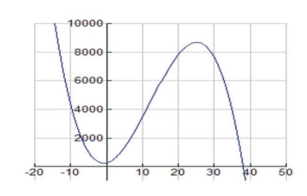
In this optimization problem, we are trying to find the maximum value of T(x). T(x) is the primary equation that will be optimized. Let’s first look at a graph of the tire function and make some observations. Set the viewing window ranges on your graphing calculator to [-10, 50] for x and [-500, 10000] for y.

The graph should appear as follows:

Screen Shot 2021-01-04 at 2.24.13 PM.png

CC BY-NC-SA

We first note that since this is a real-life application, both quantities, x and T(x), are positive or else the problem makes no sense. These conditions, together with the fact that the zero of T(x) is located at x=37.9, suggest that the actual domain of this function is 0<x≤37.9. This restricted domain, which we refer to as a feasible domain, illustrates a common feature of optimization problems: that the real-life conditions of the situation under study dictate the domain values.

We can use the calculator graph or use the First and Second Derivative Tests to find the absolute maximums and minimums on the closed interval [0, 37.9].

1^st Derivative

\[ f′(x)=−3x^2+73x+50 \nonumber\]

f′(x)=0:

at $x=− \frac{2}{3} \nonumber$ ... not in domain;

at x=25 ... in the domain.

2^nd Derivative

\[ f′′(x)=−6x+73 \nonumber\]

f′′(25)=23

There is a function maximum at x=25.

We see that the function attains an absolute maximum at x=25 at the point (25, 8687.5). So, charging a price of $25 will result in a total of 8687 tires being sold.

In many optimization problems, a secondary equation (or more than one) must be used to reduce the number of variables in the primary equation before starting the optimization procedure (use of a graphing calculator; application of derivative tests).

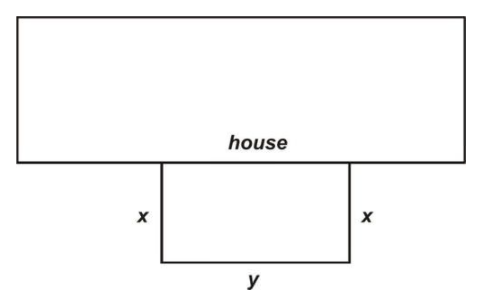
Suppose that Mary wishes to make an outdoor rectangular pen for her pet chihuahua. She would like the pen to enclose an area in her backyard with one of the sides of the rectangle made by the side of Mary's house as indicated in the following figure. If she has 90 ft of fencing to work with, what dimensions of the pen will result in the maximum area?

Screen Shot 2021-01-04 at 2.26.41 PM.png

CC BY-NC-SA

The dimensions of the pen are x and y in the figure. The primary equation is the function that models the area, A, of the pen. We wish to maximize:

\[ A=xy \nonumber\]

The secondary equation comes from the information concerning the fencing Mary has to work with. In particular,

\[ 2x+y=90 \nonumber\]

Solving for y we have

\[ y=90−2x \nonumber\]

We now substitute into the primary equation to get:

$ A=xy=x(90−2x) \nonumber$, or

$ A(x)=−2x^2+90x \nonumber$

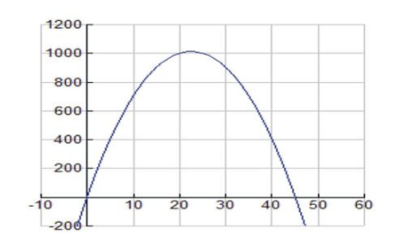
It is always helpful to view the graph of the function to be optimized. Set the viewing window ranges on your graphing calculator to [-10, 100] for x and [-500, 1200] for y. The graph should appear as follows:

Screen Shot 2021-01-04 at 2.34.06 PM.png

CC BY-NC-SA

The feasible domain of this function is 0<x<45, which makes sense because if x is 45 feet, then the figure will be two 45-foot-long fences going away from the house with 0 feet left for the width y.

We can find the solution by using the graphing calculator, and/or the First and Second Derivative Tests and the method for finding absolute maximums and minimums on a closed interval (in this problem, [0, 45]).

1^st Derivative

A′(x)=−4x+90

A′(x)=0:

at x=22.5 ... in the domain.

2^nd Derivative

A′′=−4

There is a function maximum at x=22.5.

We see that the function attains an absolute maximum at x=22.5 at the point (22.5, 1012.5).

So the dimensions of the pen should be x=22.5, and y=45; with those dimensions, the pen will enclose an area of 1012.5 ft2.

Optimization problems involving geometric shapes really help illustrate the problem solving process. Here is another:

A certain brand of lemonade sells its product in 16-ounce aluminum cans that hold 473 ml (1 ml=1 cm3). Find the dimensions of the cylindrical can that will use the least amount of aluminum.

We need to develop the formula for the surface area of the can. This consists of the top and bottom areas, each $ πr^2 \nonumber$, and the surface area of the side, $ 2πrh \nonumber$ (product of circumference of the top and height of can). Hence the primary equation is

\[ A=2πr^2+2πrh \nonumber\].

We observe that both our feasible domains require $r,h>0 \nonumber$.

To reduce the number of variables in the primary equation, we need a secondary equation that will give us a relationship between r and h. We note that the volume for a circular cylinder is given by $ V=πr^2h \nonumber$, which provides a relationship between r and h. The secondary equation is:

\[ h= \frac{V}{πr^2}= \frac{473}{πr^2} \nonumber\]

We substitute this expression for h into the primary equation to get:

$ A(r)=2πr^2+2πr( \frac{473}{πr^2}) \nonumber$, or

\[ A(r)=2πr^2+\frac{946}{r} \nonumber\].

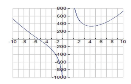
The graph of the function A(r) is shown below:

Screen Shot 2021-01-05 at 12.19.50 PM.png

CC BY-NC-SA

The feasible domain is r>0.

1^st Derivative

\[ A′(r)=4πr− \frac{946}{r^2} \nonumber\]

A′(r)=0:

at $ r= \frac{946}{4π}^{\frac{1}{3}}≈4.22 \nonumber$ cm ... in the domain.

2^nd Derivative

$ A′′(r)=4π+ \frac{1892}{r^3} \nonumber$

A′′(r)>0 for r>0

There is a function minimum at r≈4.22 cm.

Hence we have a minimum surface area of 996.2 cm2 when r≈9.06 cm and h≈8.44 cm.

Examples

Example 1

Earlier, you were asked about what dimensions will minimize the amount of metal required to construct a storage tank of volume 1000 m3 that is in the shape of a right circular cylinder and has a top that is a hemisphere.

The volume of the tank consists of the volume of a cyclinder and the volume of a hemisphere. The volume can be expressed as: $ V=πr^2h+ \frac{1}{2}( \frac{4}{3}πr^3)=1000 \nonumber$ where r is the radius of the tank (in meters), and h is the cyclinder’s height (in meters).

You would like to minimize the amount of metal used, which is the same as asking to minimize the area of the tank. This should be the optimization problem statement.

The area can be expressed as: $ A=2πrh+ \frac{1}{2}(4πr^2) \nonumber$. Because there are two variables, r and h, we should make h a function r, i.e., h(r), using the equation for V.

\[h(r)= \frac{1000}{πr^2}− \frac{2}{3}r \nonumber\)

The optimization problem statement is then:

$ \frac{dA}{dr}=0= \frac{d}{dr}[2πrh(r)+ \frac{1}{2}(4πr^2)]=2π[h(r)+r \frac{dh}{dr}+2r] \nonumber$, or

\[ h(r)+r \frac{dh}{dr}+2r=0 \nonumber\].

The next step is to solve the optimization problem to see if there is a solution that makes sense. Can you do it?

Example 2

A storage bin is to be constructed having a rectangular base, rectangular sides, and open at the top. Its width is 4 meters and its volume is 36 cubic meters. If building the bin costs $10/sq. m. for the base and $5/sq. m. for the sides, what is the cost of the least expensive bin? What are its dimensions?

Let the dimensions of the bin be l length, w width, and h height. Note that w=4 meters.

The primary equation is the function that models the cost, C, of the bin. We wish to minimize:

\[ C=10lw+5[2lh+2wh]=10[lw+lh+wh]=10[4l+lh+wh] \nonumber\]

The secondary equation comes from the information concerning the volume of the bin:

\[ V=lwh=4lh=36 \nonumber\]

Using the secondary equation in the primary equation:

\[ C=10[4l+lh+wh]=10[4l+\frac{36}{4}+\frac{36}{l}]=40[l+2.25+\frac{9}{l}] \nonumber\]

We can find the solution by using the First and Second Derivative Tests and the method for finding absolute maximums and minimums on a closed interval (in this problem, [0, 45]).

1^st Derivative	\[ C′(l)=40(1−\frac{9}{l^2}) \nonumber\]	C′(l)=0: at l=3 (in the domain) and l=−3 (not in domain).
2^nd Derivative	\[ C′′(l)=\frac{720}{l^3} \nonumber\]	C′′(3)≈26.7 . . . Cost function is concave upward. There is a function minimum at l=3.

1^st Derivative

\[ C′(l)=40(1−\frac{9}{l^2}) \nonumber\]

C′(l)=0: at l=3 (in the domain) and l=−3 (not in domain).

2^nd Derivative

\[ C′′(l)=\frac{720}{l^3} \nonumber\]

C′′(3)≈26.7 . . . Cost function is concave upward.

There is a function minimum at l=3.

So the dimensions of the bin are: l=3 meters, w=4 meters, and h=3 meters.

The cost to build the bin: C(3)=$40(3+2.25+3)=$330.

Review

For #1-4, find the absolute maximum and absolute minimum values, if they exist.

$ f(x)=2x^2−6x+6 \mbox{ on } [0, 5] \nonumber$
$ f(x)=x^3+3x^2 \mbox{ on } [-2, 3] \nonumber$
$ f(x)=3x^{\frac{2}{3}}−6x+x \mbox{ on } [1, 8] \nonumber$
$ f(x)=x^4−x^3 \mbox{ on } [-2, 2] \nonumber$
Find the dimensions of a rectangle having area $ 2000 ft^2 \nonumber$ whose perimeter is as small as possible.
Find two numbers whose product is 50 and whose sum is a minimum.
John is shooting a basketball from half-court. It is approximately 45 ft from the half court line to the hoop. The function $ s(t)=−0.025x^2+x+15 \nonumber$ models the basketball’s height above the ground s(t) in feet, when it is t feet from the hoop. How many feet from John will the ball reach its highest height? What is that height?
The height of a model rocket t seconds into flight is given by the formula $ h(t)=−13t^3+4t^2+25t+4 \nonumber$.
1. How long will it take for the rocket to attain its maximum height?
2. What is the maximum height that the rocket will reach?
3. How long will the flight last?
Show that of all rectangles of a given perimeter, the rectangle with the greatest area is a square.
Show that of all rectangles of a given area, the rectangle with the smallest perimeter is a square.
Eduardo wants to build a fence which will protect his rectangular tomato garden from the various hungry critters roaming the landscape. He purchases 100 feet of fence. What should the dimensions of the tomato garden be if it is to have the maximum area that can be contained by 100 feet of fence.
Hans has been challenged to find two nonnegative numbers whose sum is 36 so that the product of the two numbers is maximal. How should he proceed?
Lucia needs to find two nonnegative numbers whose product is 25 so that the sum of one plus the square of the other is minimized, in order to gain membership to a club. What numbers is she after?
Esmeralda wants to enclose a field with a rectangular fence to keep her goats from escaping. One side of the field is against a building, so it will not require fencing. She has 50 feet of fencing material. What are dimensions of the maximum area she can fence?
Which point on the graph of the function $ y=\sqrt{x} \nonumber$ is closest to the point (1, 0)?

Review (Answers)

To see the Review answers, open this PDF file and look for section 4.9.

Vocabulary

Term	Definition
feasible domain	The feasible domain is the subset of the domain of the primary function that can be used. This restricted domain is determined by constraints of the optimization problem.
optimal value	An optimal value or solution is the best solution to the optimization problem.
optimization	An optimization problem is a problem of finding the best solution to a problem from all the feasible solutions.
primary equation	The primary equation of an optimization problem is the function or equation for which the optimal value or solution is being sought.
secondary equation	A secondary equation is one of the equations used to relate variables of the problem and reduce the number of variables in the primary equation.