
8.3: Analyzing the Graphs of Functions
- Page ID
- 1201
\( \newcommand{\vecs}[1]{\overset { \scriptstyle \rightharpoonup} {\mathbf{#1}} } \)
\( \newcommand{\vecd}[1]{\overset{-\!-\!\rightharpoonup}{\vphantom{a}\smash {#1}}} \)
\( \newcommand{\dsum}{\displaystyle\sum\limits} \)
\( \newcommand{\dint}{\displaystyle\int\limits} \)
\( \newcommand{\dlim}{\displaystyle\lim\limits} \)
\( \newcommand{\id}{\mathrm{id}}\) \( \newcommand{\Span}{\mathrm{span}}\)
( \newcommand{\kernel}{\mathrm{null}\,}\) \( \newcommand{\range}{\mathrm{range}\,}\)
\( \newcommand{\RealPart}{\mathrm{Re}}\) \( \newcommand{\ImaginaryPart}{\mathrm{Im}}\)
\( \newcommand{\Argument}{\mathrm{Arg}}\) \( \newcommand{\norm}[1]{\| #1 \|}\)
\( \newcommand{\inner}[2]{\langle #1, #2 \rangle}\)
\( \newcommand{\Span}{\mathrm{span}}\)
\( \newcommand{\id}{\mathrm{id}}\)
\( \newcommand{\Span}{\mathrm{span}}\)
\( \newcommand{\kernel}{\mathrm{null}\,}\)
\( \newcommand{\range}{\mathrm{range}\,}\)
\( \newcommand{\RealPart}{\mathrm{Re}}\)
\( \newcommand{\ImaginaryPart}{\mathrm{Im}}\)
\( \newcommand{\Argument}{\mathrm{Arg}}\)
\( \newcommand{\norm}[1]{\| #1 \|}\)
\( \newcommand{\inner}[2]{\langle #1, #2 \rangle}\)
\( \newcommand{\Span}{\mathrm{span}}\) \( \newcommand{\AA}{\unicode[.8,0]{x212B}}\)
\( \newcommand{\vectorA}[1]{\vec{#1}} % arrow\)
\( \newcommand{\vectorAt}[1]{\vec{\text{#1}}} % arrow\)
\( \newcommand{\vectorB}[1]{\overset { \scriptstyle \rightharpoonup} {\mathbf{#1}} } \)
\( \newcommand{\vectorC}[1]{\textbf{#1}} \)
\( \newcommand{\vectorD}[1]{\overrightarrow{#1}} \)
\( \newcommand{\vectorDt}[1]{\overrightarrow{\text{#1}}} \)
\( \newcommand{\vectE}[1]{\overset{-\!-\!\rightharpoonup}{\vphantom{a}\smash{\mathbf {#1}}}} \)
\( \newcommand{\vecs}[1]{\overset { \scriptstyle \rightharpoonup} {\mathbf{#1}} } \)
\(\newcommand{\longvect}{\overrightarrow}\)
\( \newcommand{\vecd}[1]{\overset{-\!-\!\rightharpoonup}{\vphantom{a}\smash {#1}}} \)
\(\newcommand{\avec}{\mathbf a}\) \(\newcommand{\bvec}{\mathbf b}\) \(\newcommand{\cvec}{\mathbf c}\) \(\newcommand{\dvec}{\mathbf d}\) \(\newcommand{\dtil}{\widetilde{\mathbf d}}\) \(\newcommand{\evec}{\mathbf e}\) \(\newcommand{\fvec}{\mathbf f}\) \(\newcommand{\nvec}{\mathbf n}\) \(\newcommand{\pvec}{\mathbf p}\) \(\newcommand{\qvec}{\mathbf q}\) \(\newcommand{\svec}{\mathbf s}\) \(\newcommand{\tvec}{\mathbf t}\) \(\newcommand{\uvec}{\mathbf u}\) \(\newcommand{\vvec}{\mathbf v}\) \(\newcommand{\wvec}{\mathbf w}\) \(\newcommand{\xvec}{\mathbf x}\) \(\newcommand{\yvec}{\mathbf y}\) \(\newcommand{\zvec}{\mathbf z}\) \(\newcommand{\rvec}{\mathbf r}\) \(\newcommand{\mvec}{\mathbf m}\) \(\newcommand{\zerovec}{\mathbf 0}\) \(\newcommand{\onevec}{\mathbf 1}\) \(\newcommand{\real}{\mathbb R}\) \(\newcommand{\twovec}[2]{\left[\begin{array}{r}#1 \\ #2 \end{array}\right]}\) \(\newcommand{\ctwovec}[2]{\left[\begin{array}{c}#1 \\ #2 \end{array}\right]}\) \(\newcommand{\threevec}[3]{\left[\begin{array}{r}#1 \\ #2 \\ #3 \end{array}\right]}\) \(\newcommand{\cthreevec}[3]{\left[\begin{array}{c}#1 \\ #2 \\ #3 \end{array}\right]}\) \(\newcommand{\fourvec}[4]{\left[\begin{array}{r}#1 \\ #2 \\ #3 \\ #4 \end{array}\right]}\) \(\newcommand{\cfourvec}[4]{\left[\begin{array}{c}#1 \\ #2 \\ #3 \\ #4 \end{array}\right]}\) \(\newcommand{\fivevec}[5]{\left[\begin{array}{r}#1 \\ #2 \\ #3 \\ #4 \\ #5 \\ \end{array}\right]}\) \(\newcommand{\cfivevec}[5]{\left[\begin{array}{c}#1 \\ #2 \\ #3 \\ #4 \\ #5 \\ \end{array}\right]}\) \(\newcommand{\mattwo}[4]{\left[\begin{array}{rr}#1 \amp #2 \\ #3 \amp #4 \\ \end{array}\right]}\) \(\newcommand{\laspan}[1]{\text{Span}\{#1\}}\) \(\newcommand{\bcal}{\cal B}\) \(\newcommand{\ccal}{\cal C}\) \(\newcommand{\scal}{\cal S}\) \(\newcommand{\wcal}{\cal W}\) \(\newcommand{\ecal}{\cal E}\) \(\newcommand{\coords}[2]{\left\{#1\right\}_{#2}}\) \(\newcommand{\gray}[1]{\color{gray}{#1}}\) \(\newcommand{\lgray}[1]{\color{lightgray}{#1}}\) \(\newcommand{\rank}{\operatorname{rank}}\) \(\newcommand{\row}{\text{Row}}\) \(\newcommand{\col}{\text{Col}}\) \(\renewcommand{\row}{\text{Row}}\) \(\newcommand{\nul}{\text{Nul}}\) \(\newcommand{\var}{\text{Var}}\) \(\newcommand{\corr}{\text{corr}}\) \(\newcommand{\len}[1]{\left|#1\right|}\) \(\newcommand{\bbar}{\overline{\bvec}}\) \(\newcommand{\bhat}{\widehat{\bvec}}\) \(\newcommand{\bperp}{\bvec^\perp}\) \(\newcommand{\xhat}{\widehat{\xvec}}\) \(\newcommand{\vhat}{\widehat{\vvec}}\) \(\newcommand{\uhat}{\widehat{\uvec}}\) \(\newcommand{\what}{\widehat{\wvec}}\) \(\newcommand{\Sighat}{\widehat{\Sigma}}\) \(\newcommand{\lt}{<}\) \(\newcommand{\gt}{>}\) \(\newcommand{\amp}{&}\) \(\definecolor{fillinmathshade}{gray}{0.9}\)Given a set of information on the key properties of a function, you can sketch the graph. Before we proceed, make an attempt to summarize for what you think are key properties. Often, the key properties of a function are not all presented to you directly, but must be determined from the information at hand.
Analyzing Graphs of Functions
We will first summarize the kind of information about functions we now can generate based on our previous concepts. Then we will use this information to analyze examples of representative rational, polynomial, radical, and trigonometric functions.
Let's use a table like the one shown as a template to organize our findings.
| f(x)= | Analysis |
| Domain and Range | |
| Intercepts and Zeros | |
| Asymptotes and limits at infinity | |
| Differentiability | |
| Intervals where f is increasing | |
| Intervals where f is decreasing | |
| Relative extrema | |
| Concavity | |
| Inflection points |
Analyzing Rational Functions
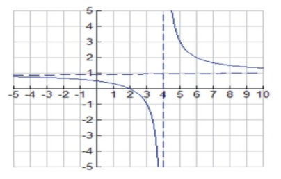
Consider the rational function \( f(x)=\frac{x^2−4}{x^2−2x−8} \nonumber\).
Zeroes, Domain, and Range
The function appears to have zeros at x=±2. However, once we factor the expression we see
\( \frac{x^2−4}{x^2−2x−8}=\frac{(x+2)(x−2)}{(x−4)(x+2)}= \frac{x−2}{x−4} \nonumber\)
Hence, the function has a zero at x=2, there is a hole in the graph at x=−2, the domain is \( (−∞,−2)∪(−2,4)∪(4,+∞) \nonumber\), and the y-intercept is at (0,12).
Asymptotes and Limits at Infinity
Given the domain, we note that there is a vertical asymptote at x=4. To determine other asymptotes, we examine the limit of f as x→∞ and x→−∞. We have
\[ \lim_{x \to ∞} \frac{x^2−4}{x^2−2x−8}= \lim_{x \to ∞} \frac{ \frac{x^2}{x^2}−\frac{4}{x^2}} {\frac{x^2}{x^2}−\frac{2x}{x^2}−\frac{8}{x^2}}=\lim_{x \to ∞} \frac{1−\frac{4}{x^2}}{1−\frac{2}{x}−\frac{8}{x^2}}=1 \nonumber\].
Similarly, we see that \( \lim_{x \to −∞} \frac{x^2−4}{x^2−2x−8}=1 \nonumber\). We also note that \( y≠\frac{2}{3} \nonumber\) since x≠−2.
Hence we have a horizontal asymptote at y=1.
Differentiability
\( f′(x)=\frac{−2x^2−8x−8}{(x2−2x−8)}=\frac{−2}{(x−4)^2}<0 \nonumber\). Hence the function is differentiable at every point of its domain, and since f′(x)<0 on its domain, then f is decreasing on its domain, \( (−∞,−2)∪(−2,4)∪(4,+∞) \nonumber\).
\[ f′′(x)= \frac{4}{(x−4)^3} \nonumber\].
f′′(x)≠0 in the domain of f. Hence there are no relative extrema and no inflection points.
Similarly, f′′(x)<0 when x<4. Hence, the graph is concave down for x<4, x≠−2.
Let’s summarize our results in the table before we sketch the graph.
| f(x)=x2−4x2−2x−8 | Analysis |
| Domain and Range |
\( D=(−∞,−2)∪(−2,4)∪(4,+∞) \nonumber\) \( R={ \mbox{ all reals }≠1or \frac{2}{3}} |
| Intercepts and Zeros |
Zero at x=2, y− intercept at (0,\( \frac{1}{2} \nonumber\)) |
| Asymptotes and limits at infinity |
VA at x=4, HA at y=1, Hole in the graph at x=−2 |
| Differentiability | Differentiable at every point of its domain |
| Intervals where f is increasing | Nowhere |
| Intervals where f is decreasing | \( (−∞,−2)∪(−2,4)∪(4,+∞) \nonumber\) |
| Relative extrema | None |
| Concavity |
Concave up in (4,+∞), Concave down in \( (−∞,−2)∪(−2,4) \nonumber\) |
| Inflection points |
None |
Finally, we sketch the graph as follows:
CC BY-NC-SA
Analyzing Radical Functions
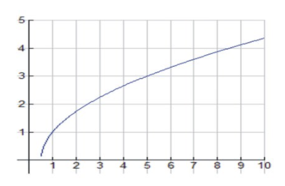
Now, Consider the function \( f(x)= \sqrt{2x−1} \nonumber\).
Zeroes, Domain, and Range
The domain of f is \( (\frac{1}{2},+∞) \nonumber\), and it has a zero at \(x=\frac{1}{2} \nonumber\).
Asymptotes and Limits at Infinity
Given the domain, we note that there are no vertical asymptotes. We note that \( \lim_{x \to ∞} f(x)=+∞ \nonumber\).
Differentiability
\( f′(x)=\frac{1}{\sqrt{2x−1}}>0 \nonumber\) for the entire domain of f. Hence f is increasing everywhere in its domain. f′(x) is not defined at \( x=\frac{1}{2} \nonumber\), so \( x=\frac{1}{2} \nonumber\) is a critical value.
\( f′′(x)=\frac{−1}{\sqrt{(2x−1)^3}<0 \nonumber\) everywhere in \( (\frac{1}{2},+∞) \nonumber\). Hence f is concave down in \( (\frac{1}{2},+∞) \nonumber\).
f′(x) is not defined at \( x=\frac{1}{2} \nonumber\), so \( x=\frac{1}{2} \nonumber\) is an absolute minimum.
| f(x)=2x‾‾√−1 | Analysis |
| Domain and Range |
\( D=(\frac{1}{2},+∞),R={y≥0} \nonumber\) |
| Intercepts and Zeros |
Zero at \( x=\frac{1}{2} \nonumber\), No y− intercept |
| Asymptotes and limits at infinity |
No asymptotes |
| Differentiability | Differentiable in (\( \frac{1}{2} \nonumber\),+∞) |
| Intervals where f is increasing | Everywhere in D=(\( \frac{1}{2} \nonumber\),+∞) |
| Intervals where f is decreasing | Nowhere |
| Relative extrema | None |
| Concavity |
Absolute minimum at x=\( \frac{1}{2} \nonumber\), located at (\( \frac{1}{2} \nonumber\),0) Concave down in (\( \frac{1}{2} \nonumber\),+∞) |
| Inflection points |
None |
Here is a sketch of the graph:
CC BY-NC-SA
Analyzing Trigonometric Functions
We will see that while trigonometric functions can be analyzed using what we know about derivatives, they will provide some interesting challenges that we will need to address.
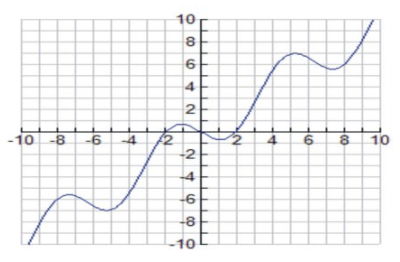
Consider the function \( f(x)=x−2sinx \nonumber\) on the interval \( [−π,π] \nonumber\).
Zeroes, Domain, and Range
We note that f is a continuous function and attains an absolute maximum and minimum in \( [−π,π] \nonumber\). Its domain is \( [−π,π] \nonumber\), and its range is \( R={−π≤y≤π} \nonumber\).
Differentiability
\[ f′(x)=1−2cosx=0 \mbox{ at } x=−\frac{π}{3},\frac{π}{3} \nonumber\].
Note that \( f′(x)>0 \mbox{ on } (−π,−\frac{π}{3}) \mbox{ and } (\frac{π}{3},π) \nonumber\); therefore the function is increasing in (−π,−π3) and (π3,π).
Note that f′(x)<0 on (−π3,π3); therefore the function is decreasing in (−π3,π3).
f′′(x)=2sinx=0 if x=0,π,−π. Hence the critical values are at x=−π,−π3,π3, and π.
f′′(π3)>0; hence there is a relative minimum at x=π3.
f′′(−π3)<0; hence there is a relative maximum at x=−π3.
f′′(x)<0 on (−π,0) and f′′(x)>0 on (0,π). Hence the graph is concave down on (−π,0) and concave up and decreasing on (0,π). There is an inflection point at x=0, located at the point (0, 0).
Finally, there is absolute minimum at \( x=−π \nonumber\), located at \( (−π,−π) \nonumber\), and an absolute maximum at \( x=π \nonumber\), located at \( (π,π) \nonumber\).
| f(x)=x−2sinx | Analysis |
| Domain and Range |
\( D=[−π,π],R={−π≤y≤π} \nonumber\) |
| Intercepts and Zeros |
\( x=−\frac{π}{3}, \frac{π}{3} \nonumber\) |
| Asymptotes and limits at infinity |
No asymptotes |
| Differentiability | Differentiable in \( D=[−π,π] \nonumber\) |
| Intervals where f is increasing | \( (\frac{π}{3},π) \mbox{ and } (−π,−\frac{π}{3}) \nonumber\) |
| Intervals where f is decreasing | \( (−\frac{π}{3},\frac{π}{3}) |
| Relative extrema |
Relative maximum at \( x=−\frac{π}{3} \nonumber\) Relative minimum at \( x=\frac{π}{3} \nonumber\) |
| Concavity |
Absolute maximum at x=π, located at (π,π) Absolute minimum at x=−π, located at (−π,−π) Concave up in (0,π) |
| Inflection points |
x=0, located at the point (0, 0) |
Here is a sketch of the graph:
CC BY-NC-SA
Examples
Example 1
Earlier, you were asked to summarize the key properties of functions. As you have seen in this concept, key properties of functions include: domain, range, intercepts, asymptotes (including limits at infinity), continuity and differentiability, increasing and decreasing intervals, extrema, concavity, and points of inflection.
Example 2
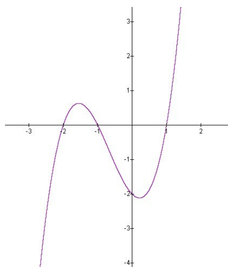
Consider the polynomial function \(f(x)=x^3+2x^2−x−2 \nonumber\).
Zeroes, Domain, and Range
The domain of f is (−∞,+∞) and the y-intercept at (0, -2).
The function can be factored \( f(x)=x^3+2x^2−x−2=x^2(x+2)−1(x+2)=(x^2−1)(x+2)=(x−1)(x+1)(x+2) \nonumber\)
and thus has zeros at x=±1,−2.
CC BY-NC-SA
Asymptotes and Limits at infinity
Given the domain, we note that there are no vertical asymptotes. We note that and \( \lim_{x \to ∞} f(x)=+∞ \mbox{ and } \lim_{x \to {−∞}} f(x)=−∞ \nonumber\).
Differentiability
\( f′(x)=3x^2+4x−1=0 \mbox{ if } x=\frac{−4±\sqrt{28}}{6}=\frac{−2±\sqrt{7}}{3} \nonumber\). These are the critical values. We note that the function is differentiable at every point of its domain.
\( f′(x)>0 \mbox{ on } (−∞,\sqrt{−2−\sqrt{7}}{3}) \mbox{ and } (\frac{−2+\sqrt{7}}{3},+∞) \nonumber\); hence the function is increasing in these intervals.
Similarly, \( f′(x)<0 \mbox{ on } (\frac{−2−\sqrt{7}}{3},\fraac{−2+\sqrt{7}}{3}) \nonumber\) and thus is f decreasing there.
\( f′′(x)=6x+4=0 \mbox{ if } x=−\frac{2}{3} \nonumber\) where there is an inflection point.
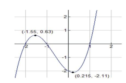
In addition, \( f′′(\frac{−2−\sqrt{7}}{3})<0 \nonumber\). Hence the graph has a relative maximum at \( x=\frac{−2−\sqrt{7}}{3} \nonumber\) and located at the point (-1.55, 0.63).
We note that \( f′′(x)<0 \mbox{ for } x<−\sqrt{2}{3} \nonumber\). The graph is concave down in \( (−∞,−\frac{2}{3}) \nonumber\).
And we have \( f′′(\frac{−2+\sqrt{7}}{3})>0 \nonumber\); hence the graph has a relative minimum at \( x=\frac{−2+\sqrt{7}}{3} \nonumber\) and located at the point (0.22, -2.11).
We note that \( f′′(x)>0 \mbox{ for } x>−\frac{2}{3} \nonumber\). The graph is concave up in \( (−\frac{2}{3},+∞) \nonumber\).
Table Summary
| \( f(x)=x^3+2x^2−x−2 \nonumber\) | Analysis |
| Domain and Range |
D=(−∞,+∞),R={all reals} |
| Intercepts and Zeros |
Zeros at x=±1,−2,y, intercepts at (0, -2) |
| Asymptotes and limits at infinity |
No asymptotes |
| Differentiability | Differentiable at every point of it's domain |
| Intervals where f is increasing | \( (−∞,\frac{−2−\sqrt{7}}{3}) and (\frac{−2+\frac{7}}{3},+∞) \nonumber\) |
| Intervals where f is decreasing | \( (\frac{−2−\sqrt{7}}{3},\frac{−2+\sqrt{7}}{3}) \nonumber\) |
| Relative extrema |
Relative maximum at \( x=\frac{−2−\sqrt{7}}{3} \nonumber\) and located at the point (-1.55, 0.63); Relative minimum at \( x=\frac{−2+\sqrt{7}}{3} \nonumber\) and located at the point (0.22, -2.11). |
| Concavity |
Concave up in \( (−\frac{2}{3},+∞) \nonumber\). Concave down in \( (−∞,−\frac{2}{3}) \nonumber\). |
| Inflection points |
\( x=−\frac{2}{3} \nonumber\), located at the point \( (−\frac{2}{3},−.74) \nonumber\) |
Here is a sketch of the graph:
CC BY-NC-SA
Review
For all of the following functions, summarize the functions by filling out the table below. Use the information to sketch a graph of the function.
| f(x)= | Analysis |
| Domain and Range | |
| Intercepts and Zeros | |
| Asymptotes and limits at infinity | |
| Differentiability | |
| Intervals where f is increasing | |
| Intervals where f is decreasing | |
| Relative extrema | |
| Concavity | |
| Inflection points |
- \( f(x)=x^3+3x^2−x−3 \nonumber\)
- \( f(x)=−x^4+4x^3−4x^2 \nonumber\)
- \( f(x)=\frac{2x−2}{x^2} \nonumber\)
- \( f(x)=x−x^{\frac{1}{3}} \nonumber\)
- \( f(x)=−\sqrt{2x−6}+3 \nonumber\)
- \( f(x)=x^2−2\sqrt{x} \nonumber\)
- \( f(x)=1+cosx \mbox{ on the interval } [−π,π] \nonumber\)
- \( f(x)=x^2−x+1 \nonumber\)
- \( f(x)=4x^3−6x^2−1 \nonumber\)
- \( f(x)=\frac{x^2}{x−1} \nonumber\)
- \( f(x)=\frac{x^2}{e^{−x}} \nonumber\)
- \( f(x)=cosx−x \nonumber\)
- \( f(x)=e^{−2x}+e^x \nonumber\)
- \( f(x)=5e^{−x}+x^3 \nonumber\)
- \( f(x)=x^5−7x^2+2 \nonumber\)
Vocabulary
| Term | Definition |
|---|---|
| Asymptotes | An asymptote is a line on the graph of a function representing a value toward which the function may approach, but does not reach (with certain exceptions). |
| concavity | Concavity describes the behavior of the slope of the tangent line of a function such that concavity is positive if the slope is increasing, negative if the slope is decreasing, and zero if the slope is constant. |
| decreasing | A function is decreasing over an interval if its y values are getting smaller over the interval. The graph will go down from left to right over the interval. |
| differentiable | A differentiable function is a function that has a derivative that can be calculated. |
| domain | The domain of a function is the set of x-values for which the function is defined. |
| increasing | A function is increasing over an interval if its y values are getting larger over the interval. The graph will go up from left to right over the interval. |
| inflection point | An inflection point is a point in the domain where concavity changes from positive to negative or negative to positive. |
| Range | The range of a function is the set of y values for which the function is defined. |
| relative extrema | The relative extrema of a function are the points of the function with y values that are the highest or lowest of a local neighborhood of the function. |
Additional Resources
PLIX: Play, Learn, Interact, eXplore - Analyzing a rational function
Video: Graphing Using Derivatives
Real World: Total Elimination