
8.2: Newton's Method
- Page ID
- 1202
\( \newcommand{\vecs}[1]{\overset { \scriptstyle \rightharpoonup} {\mathbf{#1}} } \)
\( \newcommand{\vecd}[1]{\overset{-\!-\!\rightharpoonup}{\vphantom{a}\smash {#1}}} \)
\( \newcommand{\dsum}{\displaystyle\sum\limits} \)
\( \newcommand{\dint}{\displaystyle\int\limits} \)
\( \newcommand{\dlim}{\displaystyle\lim\limits} \)
\( \newcommand{\id}{\mathrm{id}}\) \( \newcommand{\Span}{\mathrm{span}}\)
( \newcommand{\kernel}{\mathrm{null}\,}\) \( \newcommand{\range}{\mathrm{range}\,}\)
\( \newcommand{\RealPart}{\mathrm{Re}}\) \( \newcommand{\ImaginaryPart}{\mathrm{Im}}\)
\( \newcommand{\Argument}{\mathrm{Arg}}\) \( \newcommand{\norm}[1]{\| #1 \|}\)
\( \newcommand{\inner}[2]{\langle #1, #2 \rangle}\)
\( \newcommand{\Span}{\mathrm{span}}\)
\( \newcommand{\id}{\mathrm{id}}\)
\( \newcommand{\Span}{\mathrm{span}}\)
\( \newcommand{\kernel}{\mathrm{null}\,}\)
\( \newcommand{\range}{\mathrm{range}\,}\)
\( \newcommand{\RealPart}{\mathrm{Re}}\)
\( \newcommand{\ImaginaryPart}{\mathrm{Im}}\)
\( \newcommand{\Argument}{\mathrm{Arg}}\)
\( \newcommand{\norm}[1]{\| #1 \|}\)
\( \newcommand{\inner}[2]{\langle #1, #2 \rangle}\)
\( \newcommand{\Span}{\mathrm{span}}\) \( \newcommand{\AA}{\unicode[.8,0]{x212B}}\)
\( \newcommand{\vectorA}[1]{\vec{#1}} % arrow\)
\( \newcommand{\vectorAt}[1]{\vec{\text{#1}}} % arrow\)
\( \newcommand{\vectorB}[1]{\overset { \scriptstyle \rightharpoonup} {\mathbf{#1}} } \)
\( \newcommand{\vectorC}[1]{\textbf{#1}} \)
\( \newcommand{\vectorD}[1]{\overrightarrow{#1}} \)
\( \newcommand{\vectorDt}[1]{\overrightarrow{\text{#1}}} \)
\( \newcommand{\vectE}[1]{\overset{-\!-\!\rightharpoonup}{\vphantom{a}\smash{\mathbf {#1}}}} \)
\( \newcommand{\vecs}[1]{\overset { \scriptstyle \rightharpoonup} {\mathbf{#1}} } \)
\(\newcommand{\longvect}{\overrightarrow}\)
\( \newcommand{\vecd}[1]{\overset{-\!-\!\rightharpoonup}{\vphantom{a}\smash {#1}}} \)
\(\newcommand{\avec}{\mathbf a}\) \(\newcommand{\bvec}{\mathbf b}\) \(\newcommand{\cvec}{\mathbf c}\) \(\newcommand{\dvec}{\mathbf d}\) \(\newcommand{\dtil}{\widetilde{\mathbf d}}\) \(\newcommand{\evec}{\mathbf e}\) \(\newcommand{\fvec}{\mathbf f}\) \(\newcommand{\nvec}{\mathbf n}\) \(\newcommand{\pvec}{\mathbf p}\) \(\newcommand{\qvec}{\mathbf q}\) \(\newcommand{\svec}{\mathbf s}\) \(\newcommand{\tvec}{\mathbf t}\) \(\newcommand{\uvec}{\mathbf u}\) \(\newcommand{\vvec}{\mathbf v}\) \(\newcommand{\wvec}{\mathbf w}\) \(\newcommand{\xvec}{\mathbf x}\) \(\newcommand{\yvec}{\mathbf y}\) \(\newcommand{\zvec}{\mathbf z}\) \(\newcommand{\rvec}{\mathbf r}\) \(\newcommand{\mvec}{\mathbf m}\) \(\newcommand{\zerovec}{\mathbf 0}\) \(\newcommand{\onevec}{\mathbf 1}\) \(\newcommand{\real}{\mathbb R}\) \(\newcommand{\twovec}[2]{\left[\begin{array}{r}#1 \\ #2 \end{array}\right]}\) \(\newcommand{\ctwovec}[2]{\left[\begin{array}{c}#1 \\ #2 \end{array}\right]}\) \(\newcommand{\threevec}[3]{\left[\begin{array}{r}#1 \\ #2 \\ #3 \end{array}\right]}\) \(\newcommand{\cthreevec}[3]{\left[\begin{array}{c}#1 \\ #2 \\ #3 \end{array}\right]}\) \(\newcommand{\fourvec}[4]{\left[\begin{array}{r}#1 \\ #2 \\ #3 \\ #4 \end{array}\right]}\) \(\newcommand{\cfourvec}[4]{\left[\begin{array}{c}#1 \\ #2 \\ #3 \\ #4 \end{array}\right]}\) \(\newcommand{\fivevec}[5]{\left[\begin{array}{r}#1 \\ #2 \\ #3 \\ #4 \\ #5 \\ \end{array}\right]}\) \(\newcommand{\cfivevec}[5]{\left[\begin{array}{c}#1 \\ #2 \\ #3 \\ #4 \\ #5 \\ \end{array}\right]}\) \(\newcommand{\mattwo}[4]{\left[\begin{array}{rr}#1 \amp #2 \\ #3 \amp #4 \\ \end{array}\right]}\) \(\newcommand{\laspan}[1]{\text{Span}\{#1\}}\) \(\newcommand{\bcal}{\cal B}\) \(\newcommand{\ccal}{\cal C}\) \(\newcommand{\scal}{\cal S}\) \(\newcommand{\wcal}{\cal W}\) \(\newcommand{\ecal}{\cal E}\) \(\newcommand{\coords}[2]{\left\{#1\right\}_{#2}}\) \(\newcommand{\gray}[1]{\color{gray}{#1}}\) \(\newcommand{\lgray}[1]{\color{lightgray}{#1}}\) \(\newcommand{\rank}{\operatorname{rank}}\) \(\newcommand{\row}{\text{Row}}\) \(\newcommand{\col}{\text{Col}}\) \(\renewcommand{\row}{\text{Row}}\) \(\newcommand{\nul}{\text{Nul}}\) \(\newcommand{\var}{\text{Var}}\) \(\newcommand{\corr}{\text{corr}}\) \(\newcommand{\len}[1]{\left|#1\right|}\) \(\newcommand{\bbar}{\overline{\bvec}}\) \(\newcommand{\bhat}{\widehat{\bvec}}\) \(\newcommand{\bperp}{\bvec^\perp}\) \(\newcommand{\xhat}{\widehat{\xvec}}\) \(\newcommand{\vhat}{\widehat{\vvec}}\) \(\newcommand{\uhat}{\widehat{\uvec}}\) \(\newcommand{\what}{\widehat{\wvec}}\) \(\newcommand{\Sighat}{\widehat{\Sigma}}\) \(\newcommand{\lt}{<}\) \(\newcommand{\gt}{>}\) \(\newcommand{\amp}{&}\) \(\definecolor{fillinmathshade}{gray}{0.9}\)We want to look at finding the roots of a polynomial. Sometimes the polynomial cannot be easily factored, and other algebraic methods (e.g., the quadratic equation) are not applicable, or do not work. When faced with a mathematical problem that cannot be solved with simple algebraic means, calculus sometimes provides a way of finding approximate solutions.
Newton's Method
A simple example will help introduce Newton’s Method for approximating the roots of a polynomial equation.
Let's say you want to compute \( \sqrt{5} \nonumber\) without using a calculator or a table. Any ideas how this could be done? Try thinking about this problem in a different way, so that you make use of linearization.
Assume that we are interested in solving the quadratic equation:
\[ f(x)=x^2−5=0 \nonumber\]
We know this equation has the roots \( x=± \sqrt{5} \nonumber\).
The idea here is to find the linearization of f(x) at an appropriate point, and then solve the linear equation for x. This is an added twist to the linearization problem!
How to choose the linearization point? Since \( \sqrt{4}<\sqrt{5}<\sqrt{9} \nonumber\), this mean \( 2<\sqrt{5}<3 \nonumber\).
We choose the linear approximation of f(x) to be near \( x_0=2 \nonumber\) (but, \( x_0=3 \nonumber\) could also could be selected).
\[ f(x)=x^2−5 \mbox{ and } f(2)=−1 \nonumber\]
\[ f′(x)=2x \mbox{ and } f′(2)=4 \nonumber\]
Using the linear approximation formula,
\[ f(x)≈f(x_0)+f′(x_0)(x−x_0) \nonumber\]
\[ ≈−1+(4)(x−2) \nonumber\]
\[ ≈−1+4x−8 \nonumber\]
\[ ≈4x−9 \nonumber\]
Notice that this equation is much easier to solve than \( f(x)=x^2−5=0 \nonumber\).
Setting f(x)=0 and solving for x, we obtain,
\[ 4x−9=0 \nonumber\]
\[ x=\frac{9}{4} \nonumber\]
\[ =2.25 \nonumber\]
This is a fairly good approximation, since a calculator would give x=2.23607, lower by 0.014. We can actually make this approximation to the root of f(x) even better by repeating what we have just done but using the latest estimate \( x_1=2.25= \frac{9}{4} \nonumber\), a number that is even closer to the actual value of \( \sqrt{5} \nonumber\).
\[ f(x)=x^2−5 \mbox{ and } f(2.25)=\frac{1}{16} \nonumber\]
\[ f′(x)=2x \mbox{ and } f′(2)= \frac{9}{2} \nonumber\]
Using the linear approximation again,
\[ f(x)≈f(x_1)+f′(x_1)(x−x_1) \nonumber\]
\[ ≈ \frac{1}{16}+\frac{9}{2}(x−\frac{9}{4}) \nonumber\]
\[ ≈\frac{9}{2}x−\frac{161}{16} \nonumber\].
Solving for x by setting f(x)=0, we obtain
\[ x=x_2=\frac{161}{72}=2.23611 \nonumber\]
which is an even better approximation than \[ x_1=\frac{9}{4} \nonumber\].
We could continue this process generating a better approximation to \( \sqrt{5} \nonumber\), as shown in the table, where the last estimate approximates the correct answer to 5 places. Thank goodness for calculators!
|
n |
\( x_n \nonumber\) |
\( f(x_n) \nonumber\) |
\( f′(x-n) \nonumber\) |
\( \frac{f(x_n)}{f′(x_n)} \nonumber\) |
\( x_n−\frac{f(x_n)}{f′(x_n)} \nonumber\) |
|
1 |
2 |
-1 |
4 |
-0.25 |
2.25 |
|
2 |
2.25 |
0.0625 |
4.5 |
0.01389 |
2.23611 |
|
3 |
2.23611 |
0.00019 |
4.47222 |
0.00004 |
2.23607 |
|
4 |
2.23607 |
-- |
-- |
-- |
-- |
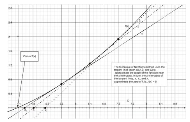
This is the basic idea of Newton’s Method. Here is a summary of the method:
- Given the function f(x), find f′(x).
- Estimate the first approximation, x0, to a solution of the equation f(x)=0. Use a graph to help in finding the first approximation if necessary (see Figure below).
- Use the current approximation xn to find the next approximation, xn+1, by using the recursion relation.
\[ x_{n+1}=x_n−\frac{f(x_n)}{f′(x_n)} \nonumber\].
- Repeat the previous step until the desired level of convergence occurs.
Note that in some cases, Newton’s Method does not converge.
CC BY-NC-SA
Examples
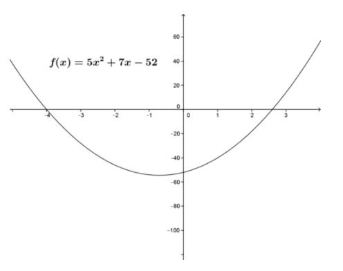
Example 1
Compare the solutions to f(x)=5x2+7x−52 in the interval [2, 3] from using the Quadratic formula and using Newton’s Method.
The function is shown in the figure.
For f(x)=5x2+7x−52=0, use of the quadratic formula gives the exact solution x=2.6 in the interval.
CC BY-NC-SA
Use of Newton’s Method with an initial estimate of x0=3, yields the results shown in the table.
|
n |
\( x_n \nonumber\) |
\( f(x_n) \nonumber\) |
\( f′(x-n) \nonumber\) |
\( \frac{f(x_n)}{f′(x_n)} \nonumber\) |
\( x_n−\frac{f(x_n)}{f′(x_n)} \nonumber\) |
|
1 |
3 |
14 |
37 |
0.3784 |
2.6216 |
|
2 |
2.6216 |
0.7151 |
33.216 |
0.0215 |
2.6001 |
|
3 |
2.6001 |
0.0033 |
33.001 |
0.0001 |
2.6000 |
|
4 |
2.6000 |
-- |
-- |
-- |
-- |
The technique rapidly converges to a solution.
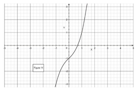
Example 2
Use Newton’s method to find the roots of the polynomial \( f(x)=x^3+x−1 \nonumber\).
The problem is to solve the equation \( f(x)=x^3+x−1=0 \nonumber\).
The equations we need are:
\[ f(x)=x^3+x−1 \nonumber\]
\[ f′(x)=3x^2+1 \nonumber\].
Using the recursion relation,
\[ x_{n+1}=x_n−\frac{f(x_n)}{f′(x_n)} \nonumber\]
\[ =x_n−\frac{x^3_n+x_n−1}{3x^2_n+1} \nonumber\].
To help us find the first approximation, we make a graph of f(x). As the figure suggests, set \( x_1=0.6 \nonumber\).
CC BY-NC-SA
Then using the recursion relation, we can generate x1:
\[ x_{n+1}=x_n−\frac{x^3_n+x_n−1}{3x^2_n+1} \nonumber\]
\[ x_2=0.6−\frac{(0.6)^3+(0.6)−1}{3(0.6)^2+1} \nonumber\]
\[ =0.6884615 \nonumber\].
By using the recursion relation several times, we can find x3 and x4 as shown in the table.
|
n |
\( x_n \nonumber\) |
\( f(x_n) \nonumber\) |
\( f′(x-n) \nonumber\) |
\( \frac{f(x_n)}{f′(x_n)} \nonumber\) |
\( x_n−\frac{f(x_n)}{f′(x_n)} \nonumber\) |
|
1 |
0.6 |
-0.184 |
2.08 |
-0.0884615 |
0.6884615 |
|
2 |
0.6884615 |
0.01477796 |
2.4219377 |
0.0061017 |
0.6823598 |
|
3 |
0.6823598 |
0.00007669 |
2.3968445 |
0.0000320 |
0.6823278 |
|
4 |
0.6823278 |
-- |
-- |
-- |
-- |
We conclude that the solution to the equation \[ x^3+x−1=0 \nonumber\] is about 0.6823.
Example 3
Use Newton’s Method to show to find the root of \( f(x)=cos(2x)−x \nonumber\).
The equations we need are:
\( f(x)=cos(2x)−x \nonumber\)
\( f(x)=−2sin(2x)−1 \nonumber\)
Using the recursion relation,
x_{n+1}=x_n\frac{f(x_n)}{f′(x_n)} \nonumber\)
\( =x_n−\frac{cos(2x_n)−x_n}{−2sin(2x_n)−1} \nonumber\)
To help us find the first approximation, we make a graph of f(x). As the figure suggests, set the first estimate at 0.5.
CC BY-NC-SA
Using the recursion relation several times gives the table values:
|
n |
\( x_n \nonumber\) |
\( f(x_n) \nonumber\) |
\( \frac{f(x_n)}{f′(xn)} \nonumber\) |
|
1 |
0.500000 |
0.0403023 |
-0.015216_8 |
|
2 |
0.515022 |
-0.0002400 |
0.0000884 |
|
3 |
0.514933 |
-0.0000000 |
0.0000000 |
|
4 |
0.514933 |
-- |
-- |
We conclude that the solution to the equation cos(2x)−x=0 is 0.514933.
Review
For all the problems, use Newton’s Method to find the roots.
- \( x^3+3=0 \nonumber\).
- \( −x+3\sqrt{−1+x}=0 \nonumber\).
- \( 4x^2−x−2 \mbox{ in the interval } [-1, 0] \nonumber\).
- \( 4x^3−6x^2−1 \nonumber\).
- \( 5e^{−x}+x^3 \nonumber\).
- \( cosx−x \nonumber\).
- \( x^5−7x^2+2 \mbox{ in the interval} [-1, 0] \nonumber\).
- \( x^5−7x^2+2 \mbox{ in the interval } [0, 1] \nonumber\).
- \( x^2cosx−x \mbox{ in the interval } [4, 5] \nonumber\).
- \( x^2cosx−x \mbox{ in the interval } [7, 8] \nonumber\).
- \( f(x)=x−2sin(x) \mbox{ to five decimal places, starting with initial guess } x_0=3 \nonumber\).
- \( f(x)=6x^3−4x+1 \nonumber\) to three decimal places, starting with initial guess \( x_0=1.2 \nonumber\).
- \( f(x)=ln(x)×(ln(x)+4)+1 \nonumber\) to five decimal places, starting with initial guess \( x_0=1 \nonumber\).
- \( f(x)=tan(x)−csc(x) \nonumber\) to six digits of accuracy, starting with initial guess \( x_0=0.7 \nonumber\).
- \( f(x)=tan^{−1}(x)+cos(x) \nonumber\) to four digits of accuracy, starting with initial guess \( x_0=−2 \nonumber\).
Vocabulary
| Term | Definition |
|---|---|
| Newton's method | Newton’s method is an iterative procedure for computing the root of an equation. |
Additional Resources
PLIX: Play, Learn, Interact, eXplore - Newton's Method
Video: Newton's Method for Solving Equations
Practice: Newton's Method
Real World: Getting to the Root of Things