1.20: Polygon Classification in the Coordinate Plane
- Page ID
- 2134
\( \newcommand{\vecs}[1]{\overset { \scriptstyle \rightharpoonup} {\mathbf{#1}} } \)
\( \newcommand{\vecd}[1]{\overset{-\!-\!\rightharpoonup}{\vphantom{a}\smash {#1}}} \)
\( \newcommand{\dsum}{\displaystyle\sum\limits} \)
\( \newcommand{\dint}{\displaystyle\int\limits} \)
\( \newcommand{\dlim}{\displaystyle\lim\limits} \)
\( \newcommand{\id}{\mathrm{id}}\) \( \newcommand{\Span}{\mathrm{span}}\)
( \newcommand{\kernel}{\mathrm{null}\,}\) \( \newcommand{\range}{\mathrm{range}\,}\)
\( \newcommand{\RealPart}{\mathrm{Re}}\) \( \newcommand{\ImaginaryPart}{\mathrm{Im}}\)
\( \newcommand{\Argument}{\mathrm{Arg}}\) \( \newcommand{\norm}[1]{\| #1 \|}\)
\( \newcommand{\inner}[2]{\langle #1, #2 \rangle}\)
\( \newcommand{\Span}{\mathrm{span}}\)
\( \newcommand{\id}{\mathrm{id}}\)
\( \newcommand{\Span}{\mathrm{span}}\)
\( \newcommand{\kernel}{\mathrm{null}\,}\)
\( \newcommand{\range}{\mathrm{range}\,}\)
\( \newcommand{\RealPart}{\mathrm{Re}}\)
\( \newcommand{\ImaginaryPart}{\mathrm{Im}}\)
\( \newcommand{\Argument}{\mathrm{Arg}}\)
\( \newcommand{\norm}[1]{\| #1 \|}\)
\( \newcommand{\inner}[2]{\langle #1, #2 \rangle}\)
\( \newcommand{\Span}{\mathrm{span}}\) \( \newcommand{\AA}{\unicode[.8,0]{x212B}}\)
\( \newcommand{\vectorA}[1]{\vec{#1}} % arrow\)
\( \newcommand{\vectorAt}[1]{\vec{\text{#1}}} % arrow\)
\( \newcommand{\vectorB}[1]{\overset { \scriptstyle \rightharpoonup} {\mathbf{#1}} } \)
\( \newcommand{\vectorC}[1]{\textbf{#1}} \)
\( \newcommand{\vectorD}[1]{\overrightarrow{#1}} \)
\( \newcommand{\vectorDt}[1]{\overrightarrow{\text{#1}}} \)
\( \newcommand{\vectE}[1]{\overset{-\!-\!\rightharpoonup}{\vphantom{a}\smash{\mathbf {#1}}}} \)
\( \newcommand{\vecs}[1]{\overset { \scriptstyle \rightharpoonup} {\mathbf{#1}} } \)
\(\newcommand{\longvect}{\overrightarrow}\)
\( \newcommand{\vecd}[1]{\overset{-\!-\!\rightharpoonup}{\vphantom{a}\smash {#1}}} \)
\(\newcommand{\avec}{\mathbf a}\) \(\newcommand{\bvec}{\mathbf b}\) \(\newcommand{\cvec}{\mathbf c}\) \(\newcommand{\dvec}{\mathbf d}\) \(\newcommand{\dtil}{\widetilde{\mathbf d}}\) \(\newcommand{\evec}{\mathbf e}\) \(\newcommand{\fvec}{\mathbf f}\) \(\newcommand{\nvec}{\mathbf n}\) \(\newcommand{\pvec}{\mathbf p}\) \(\newcommand{\qvec}{\mathbf q}\) \(\newcommand{\svec}{\mathbf s}\) \(\newcommand{\tvec}{\mathbf t}\) \(\newcommand{\uvec}{\mathbf u}\) \(\newcommand{\vvec}{\mathbf v}\) \(\newcommand{\wvec}{\mathbf w}\) \(\newcommand{\xvec}{\mathbf x}\) \(\newcommand{\yvec}{\mathbf y}\) \(\newcommand{\zvec}{\mathbf z}\) \(\newcommand{\rvec}{\mathbf r}\) \(\newcommand{\mvec}{\mathbf m}\) \(\newcommand{\zerovec}{\mathbf 0}\) \(\newcommand{\onevec}{\mathbf 1}\) \(\newcommand{\real}{\mathbb R}\) \(\newcommand{\twovec}[2]{\left[\begin{array}{r}#1 \\ #2 \end{array}\right]}\) \(\newcommand{\ctwovec}[2]{\left[\begin{array}{c}#1 \\ #2 \end{array}\right]}\) \(\newcommand{\threevec}[3]{\left[\begin{array}{r}#1 \\ #2 \\ #3 \end{array}\right]}\) \(\newcommand{\cthreevec}[3]{\left[\begin{array}{c}#1 \\ #2 \\ #3 \end{array}\right]}\) \(\newcommand{\fourvec}[4]{\left[\begin{array}{r}#1 \\ #2 \\ #3 \\ #4 \end{array}\right]}\) \(\newcommand{\cfourvec}[4]{\left[\begin{array}{c}#1 \\ #2 \\ #3 \\ #4 \end{array}\right]}\) \(\newcommand{\fivevec}[5]{\left[\begin{array}{r}#1 \\ #2 \\ #3 \\ #4 \\ #5 \\ \end{array}\right]}\) \(\newcommand{\cfivevec}[5]{\left[\begin{array}{c}#1 \\ #2 \\ #3 \\ #4 \\ #5 \\ \end{array}\right]}\) \(\newcommand{\mattwo}[4]{\left[\begin{array}{rr}#1 \amp #2 \\ #3 \amp #4 \\ \end{array}\right]}\) \(\newcommand{\laspan}[1]{\text{Span}\{#1\}}\) \(\newcommand{\bcal}{\cal B}\) \(\newcommand{\ccal}{\cal C}\) \(\newcommand{\scal}{\cal S}\) \(\newcommand{\wcal}{\cal W}\) \(\newcommand{\ecal}{\cal E}\) \(\newcommand{\coords}[2]{\left\{#1\right\}_{#2}}\) \(\newcommand{\gray}[1]{\color{gray}{#1}}\) \(\newcommand{\lgray}[1]{\color{lightgray}{#1}}\) \(\newcommand{\rank}{\operatorname{rank}}\) \(\newcommand{\row}{\text{Row}}\) \(\newcommand{\col}{\text{Col}}\) \(\renewcommand{\row}{\text{Row}}\) \(\newcommand{\nul}{\text{Nul}}\) \(\newcommand{\var}{\text{Var}}\) \(\newcommand{\corr}{\text{corr}}\) \(\newcommand{\len}[1]{\left|#1\right|}\) \(\newcommand{\bbar}{\overline{\bvec}}\) \(\newcommand{\bhat}{\widehat{\bvec}}\) \(\newcommand{\bperp}{\bvec^\perp}\) \(\newcommand{\xhat}{\widehat{\xvec}}\) \(\newcommand{\vhat}{\widehat{\vvec}}\) \(\newcommand{\uhat}{\widehat{\uvec}}\) \(\newcommand{\what}{\widehat{\wvec}}\) \(\newcommand{\Sighat}{\widehat{\Sigma}}\) \(\newcommand{\lt}{<}\) \(\newcommand{\gt}{>}\) \(\newcommand{\amp}{&}\) \(\definecolor{fillinmathshade}{gray}{0.9}\)
Parker is taking her first drawing class, though she doesn't have high hopes. When she walks into class the first day, her art teacher pulls up a picture of a cityscape and tells them that they will all be able to draw this by the end of the week. Her teacher gives them each a copy of this picture and tells them that their first assignment is to break the picture into its underlying shapes. Parker is utterly confused and overwhelmed. How can Parker figure out how to break the picture into shapes?
In this concept, you will learn how to graph geometric figures given coordinates of vertices and identify graphed figures.
Classifying Polygons in the Coordinate Plane
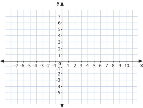
A coordinate grid is a grid in which points are graphed. It usually has two or more intersecting lines which divide a plane into quadrants, and in which ordered pairs, or coordinates, are defined. It usually has four quadrants, or sections, to it.
 Figure \(\PageIndex{2}\)
The origin is the place where the two lines intersect. Its coordinates are defined as \((0,0)\).
The \(x\)-axis is the line running from left to right that has the numbers defined on it and is usually labeled with an "\(x\)". The \(x\)-coordinate of an ordered pair is found with relation to it. All the points located on the \(x\)-axis have a \(y\)-coordinate of 0.
The \(y\)-axis is the central line that runs up-down and is labeled with a "\(y\)". Y-coordinates are plotted in reference to this axis. Again, all the \(x\)-coordinates of points located on the \(y\)-axis are 0.
An ordered pair is a list of two numbers in parenthesis, separated by a comma like this: \((5,-3)\). It tells where a point is located on the coordinate plane. The first number is the \(x\)-coordinate. It tells you where to go on the \(x\)-axis. If it is positive, you go to the right. If it is negative, you go to the left. The second number is the y-coordinate. It tells you where to go on the \(y\)-axis. If it is positive, you go up. If it is negative, you go down.
The vertex of a shape is the place where two sides of the shape come together. In general, when a shape is defined inside of a coordinate plane, it is defined by the vertices, and then the lines are drawn to connect them.
A polygon is any shape made up of rectilineal, or straight, lines. The smallest polygon is a triangle, which has three sides. A five-sided figure is a pentagon. And many polygons with more sides than five are also named.
A right angle is an angle that looks like where the axes on the coordinate plane meet.
Parallel lines are lines that will go on forever but will never converge.
The category of four-sided polygons includes:
- the square, which has four sides of equal length and its angles are all right angles;
- the rhombus which, like the square, has four equal sides, but is "tilty";
- the rectangle which has two pairs of sides which are equal and all its angles are right angles;
- the trapezoid which may have no equal sides, but it has two lines which are parallel; and
- the parallelogram which has two sets of parallel lines which are equal in length to each other (but like the rhombus, it is "tilty").
In order to graph a figure in the coordinate plane, you just graph each of the vertices and then connect them with straight lines so that none of the lines cross. The number of sides you have is the same as the number of vertices. So a triangle, for example, is defined with three vertices.
Here is an example.
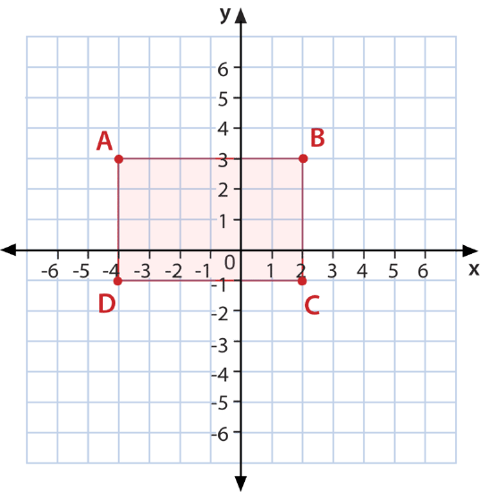
Graph a figure with the coordinates \(A(−4, 3) B(2, 3) C(2,−1) D(−4,−1)\). When finished, name the figure that has been drawn on the grid.
First, plot each point on the coordinate grid and then connect the lines.
 Figure \(\PageIndex{3}\)
Next, in order to determine what kind of shape it is, first count the number of vertices.
This figure has four, so it is one of the four-sided shapes.
Then, look to see how many of the sides are equal.
In this case, side \(AB=DC\) and \(AD=BC\). Since there are two sets of equal sides, this is either a rectangle or a parallelogram.
Finally, check the angles.
In this shape, the angles are right angles, so this is a rectangle.
Here is another example.
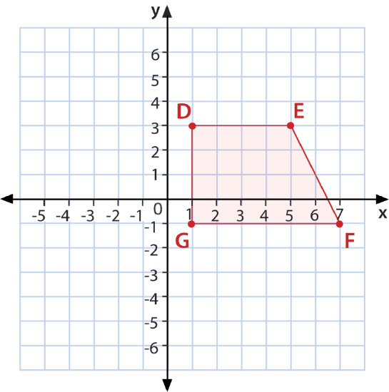
Graph and name the following figure with these coordinates \(D(1,3) E(5,3) F(7,−1) G(1,−1)\).
 Figure \(\PageIndex{4}\)
First, plot the vertices and connect them.
Next, count the number of vertices.
There are four, so this is a four-sided figure, which you can see from its shape.
Then, look at the sides.
None of the sides are the same length, so this shape must be a trapezoid.
Example \(\PageIndex{1}\)
Earlier, you were given a problem about Parker and her math-art panic attack.
Her art teacher gives her a picture of buildings in perspective and tells her to break it into its constituent shapes.
Solution
First, she draws a \(y\)-axis down the center of the back building in the picture, which looks about halfway across the picture. Then, she draws the \(x\)-axis as the horizon line.
Next, she squints at the picture and tries to see it not as buildings, but as shapes, instead. On the right side of the picture, she realizes that the buildings make a triangle with one vertex starting at the origin. And on the left of the \(y\)-axis, the other side of buildings make another triangle, also with a vertex at the origin. Even the street, she realizes, makes its own triangle, again with one vertex at the origin. And then the sky finishes it with a forth triangle with a vertex at the origin.
Then, she sees that the rest of the picture is just made up of rectangles. There is one below the street triangle, and one on the left buildings. And one where the tiny back building is.
Parker concludes that she might be able to learn to draw after all.
Example \(\PageIndex{2}\)
Determine the shape given by the following vertices.
\((−4,6)(4,6)(0,−6)\)
Solution
First, count the number of vertices.
In this case, there are three vertices. If there are three vertices, then the shape has three sides.
Next, determine which shapes are possible.
There is only one closed shape with three sides, and that is a triangle.
The answer is a triangle.
Example \(\PageIndex{3}\)
Determine the shape given by the following vertices.
\((0,2)(2,0)(0,−3)\)
Solution
First, count the number of vertices.
In this case, there are three vertices. If there are three vertices, then there are three sides.
Next, determine which shapes are possible.
There is only one closed shape with three sides, and that is a triangle.
The answer is a triangle.
Example \(\PageIndex{4}\)
Determine the shape given by the following vertices.
\((−1,−3)(−5,−3)(−7,1)(−1,1)\)
Solution
First, count the number of vertices.
In this case, there are four vertices. If there are four vertices, then the shape has four sides.
Next, determine which shapes are possible.
The four-sided figures are: square, rhombus, trapezoid, rectangle, and parallelogram.
Then, plot the vertices on a coordinate plane.
Then, determine the properties of the shape.
In this case, the shape has two parallel lines and two non-parralel lines. The only four sides figure in which that is the case is the trapezoid.
The answer is a trapezoid.
Example \(\PageIndex{5}\)
Determine the shape given by the following vertices.
\((3,3)(0,3)(0,0)(3,0)\)
Solution
First, count the number of vertices.
In this case, there are four vertices. If there are four vertices, then the shape has four sides.
Next, determine which shapes are possible.
The four-sided figures are: square, rhombus, trapezoid, rectangle, and parallelogram.
Then, plot the vertices on a coordinate plane.
Then, determine the properties of the shape.
In this case, the shape has two sets of parallel lines and and all the sides are the same length. Additionally, the shape has four right angles. The square is the shape that meets these criterion.
The answer is a square.
Review
Graph each figure using the vertices. Then name the graphed figure.
- \(A(−2,2);B(2,2);C(2,−2);D(−2,−2)\)
- \(D(−4,3);E(−1,1);F(−4,1)\)
- \((1,1)(2,3)(4,1)\)
- \((−1,3)(−5,3)(−1,0)(−5,0)\)
- \((0,5)(3,5)(0,9)(3,9)\)
- \((0,6)(2,6)(0,10)(2,10)\)
- \((−3,6)(6,0)(9,0)\)
- \((−1,6)(−1,8)(−9,6)(−9,8)\)
- \((0,−8)(1,−5)(5,−5)(4,−8)\)
- \((12,0)(12,6)(7,0)\)
For 11 - 15 draw five of your own figures on a coordinate grid. Write out each set of coordinates and work with a partner to identify each figure using only the coordinates.
Review (Answers)
To see the Review answers, open this PDF file and look for section 11.15.
Vocabulary
| Term | Definition |
|---|---|
| \(x\)-axis | The \(x\)-axis is the horizontal axis in the coordinate plane, commonly representing the value of the input or independent variable. |
| y axis | The \(y\)-axis is the vertical number line of the Cartesian plane. |
| Coordinates | The coordinates of a point represent the point's location on the Cartesian plane. Coordinates are written in ordered pairs: \(x,y)\). |
| Ordered Pair | An ordered pair, \(x,y)\), describes the location of a point on a coordinate grid. |
| Origin | The origin is the point of intersection of the x and y axes on the Cartesian plane. The coordinates of the origin are \((0, 0)\). |
| Quadrants | A quadrant is one-fourth of the coordinate plane. The four quadrants are numbered using Roman Numerals I, II, III, and IV, starting in the top-right, and increasing counter-clockwise. |
Additional Resources
Interactive Element
Video: Plotting Points on the Coordinate Plane
Practice: Polygon Classification in the Coordinate Plane

