2.11 Oblique Asymptotes
- Page ID
- 13716
\( \newcommand{\vecs}[1]{\overset { \scriptstyle \rightharpoonup} {\mathbf{#1}} } \)
\( \newcommand{\vecd}[1]{\overset{-\!-\!\rightharpoonup}{\vphantom{a}\smash {#1}}} \)
\( \newcommand{\dsum}{\displaystyle\sum\limits} \)
\( \newcommand{\dint}{\displaystyle\int\limits} \)
\( \newcommand{\dlim}{\displaystyle\lim\limits} \)
\( \newcommand{\id}{\mathrm{id}}\) \( \newcommand{\Span}{\mathrm{span}}\)
( \newcommand{\kernel}{\mathrm{null}\,}\) \( \newcommand{\range}{\mathrm{range}\,}\)
\( \newcommand{\RealPart}{\mathrm{Re}}\) \( \newcommand{\ImaginaryPart}{\mathrm{Im}}\)
\( \newcommand{\Argument}{\mathrm{Arg}}\) \( \newcommand{\norm}[1]{\| #1 \|}\)
\( \newcommand{\inner}[2]{\langle #1, #2 \rangle}\)
\( \newcommand{\Span}{\mathrm{span}}\)
\( \newcommand{\id}{\mathrm{id}}\)
\( \newcommand{\Span}{\mathrm{span}}\)
\( \newcommand{\kernel}{\mathrm{null}\,}\)
\( \newcommand{\range}{\mathrm{range}\,}\)
\( \newcommand{\RealPart}{\mathrm{Re}}\)
\( \newcommand{\ImaginaryPart}{\mathrm{Im}}\)
\( \newcommand{\Argument}{\mathrm{Arg}}\)
\( \newcommand{\norm}[1]{\| #1 \|}\)
\( \newcommand{\inner}[2]{\langle #1, #2 \rangle}\)
\( \newcommand{\Span}{\mathrm{span}}\) \( \newcommand{\AA}{\unicode[.8,0]{x212B}}\)
\( \newcommand{\vectorA}[1]{\vec{#1}} % arrow\)
\( \newcommand{\vectorAt}[1]{\vec{\text{#1}}} % arrow\)
\( \newcommand{\vectorB}[1]{\overset { \scriptstyle \rightharpoonup} {\mathbf{#1}} } \)
\( \newcommand{\vectorC}[1]{\textbf{#1}} \)
\( \newcommand{\vectorD}[1]{\overrightarrow{#1}} \)
\( \newcommand{\vectorDt}[1]{\overrightarrow{\text{#1}}} \)
\( \newcommand{\vectE}[1]{\overset{-\!-\!\rightharpoonup}{\vphantom{a}\smash{\mathbf {#1}}}} \)
\( \newcommand{\vecs}[1]{\overset { \scriptstyle \rightharpoonup} {\mathbf{#1}} } \)
\(\newcommand{\longvect}{\overrightarrow}\)
\( \newcommand{\vecd}[1]{\overset{-\!-\!\rightharpoonup}{\vphantom{a}\smash {#1}}} \)
\(\newcommand{\avec}{\mathbf a}\) \(\newcommand{\bvec}{\mathbf b}\) \(\newcommand{\cvec}{\mathbf c}\) \(\newcommand{\dvec}{\mathbf d}\) \(\newcommand{\dtil}{\widetilde{\mathbf d}}\) \(\newcommand{\evec}{\mathbf e}\) \(\newcommand{\fvec}{\mathbf f}\) \(\newcommand{\nvec}{\mathbf n}\) \(\newcommand{\pvec}{\mathbf p}\) \(\newcommand{\qvec}{\mathbf q}\) \(\newcommand{\svec}{\mathbf s}\) \(\newcommand{\tvec}{\mathbf t}\) \(\newcommand{\uvec}{\mathbf u}\) \(\newcommand{\vvec}{\mathbf v}\) \(\newcommand{\wvec}{\mathbf w}\) \(\newcommand{\xvec}{\mathbf x}\) \(\newcommand{\yvec}{\mathbf y}\) \(\newcommand{\zvec}{\mathbf z}\) \(\newcommand{\rvec}{\mathbf r}\) \(\newcommand{\mvec}{\mathbf m}\) \(\newcommand{\zerovec}{\mathbf 0}\) \(\newcommand{\onevec}{\mathbf 1}\) \(\newcommand{\real}{\mathbb R}\) \(\newcommand{\twovec}[2]{\left[\begin{array}{r}#1 \\ #2 \end{array}\right]}\) \(\newcommand{\ctwovec}[2]{\left[\begin{array}{c}#1 \\ #2 \end{array}\right]}\) \(\newcommand{\threevec}[3]{\left[\begin{array}{r}#1 \\ #2 \\ #3 \end{array}\right]}\) \(\newcommand{\cthreevec}[3]{\left[\begin{array}{c}#1 \\ #2 \\ #3 \end{array}\right]}\) \(\newcommand{\fourvec}[4]{\left[\begin{array}{r}#1 \\ #2 \\ #3 \\ #4 \end{array}\right]}\) \(\newcommand{\cfourvec}[4]{\left[\begin{array}{c}#1 \\ #2 \\ #3 \\ #4 \end{array}\right]}\) \(\newcommand{\fivevec}[5]{\left[\begin{array}{r}#1 \\ #2 \\ #3 \\ #4 \\ #5 \\ \end{array}\right]}\) \(\newcommand{\cfivevec}[5]{\left[\begin{array}{c}#1 \\ #2 \\ #3 \\ #4 \\ #5 \\ \end{array}\right]}\) \(\newcommand{\mattwo}[4]{\left[\begin{array}{rr}#1 \amp #2 \\ #3 \amp #4 \\ \end{array}\right]}\) \(\newcommand{\laspan}[1]{\text{Span}\{#1\}}\) \(\newcommand{\bcal}{\cal B}\) \(\newcommand{\ccal}{\cal C}\) \(\newcommand{\scal}{\cal S}\) \(\newcommand{\wcal}{\cal W}\) \(\newcommand{\ecal}{\cal E}\) \(\newcommand{\coords}[2]{\left\{#1\right\}_{#2}}\) \(\newcommand{\gray}[1]{\color{gray}{#1}}\) \(\newcommand{\lgray}[1]{\color{lightgray}{#1}}\) \(\newcommand{\rank}{\operatorname{rank}}\) \(\newcommand{\row}{\text{Row}}\) \(\newcommand{\col}{\text{Col}}\) \(\renewcommand{\row}{\text{Row}}\) \(\newcommand{\nul}{\text{Nul}}\) \(\newcommand{\var}{\text{Var}}\) \(\newcommand{\corr}{\text{corr}}\) \(\newcommand{\len}[1]{\left|#1\right|}\) \(\newcommand{\bbar}{\overline{\bvec}}\) \(\newcommand{\bhat}{\widehat{\bvec}}\) \(\newcommand{\bperp}{\bvec^\perp}\) \(\newcommand{\xhat}{\widehat{\xvec}}\) \(\newcommand{\vhat}{\widehat{\vvec}}\) \(\newcommand{\uhat}{\widehat{\uvec}}\) \(\newcommand{\what}{\widehat{\wvec}}\) \(\newcommand{\Sighat}{\widehat{\Sigma}}\) \(\newcommand{\lt}{<}\) \(\newcommand{\gt}{>}\) \(\newcommand{\amp}{&}\) \(\definecolor{fillinmathshade}{gray}{0.9}\)When the degree of the numerator of a rational function exceeds the degree of the denominator by one then the function has oblique asymptotes. In order to find these asymptotes, you need to use polynomial long division and the non-remainder portion of the function becomes the oblique asymptote. A natural question to ask is: what happens when the degree of the numerator exceeds that of the denominator by more than one?
Oblique Asymptotes
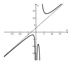
The following function is shown before and after polynomial long division is performed.
\(f(x)=\frac{x^{4}+3 x^{2}+2 x+14}{x^{3}-3 x^{2}}=x+3+\frac{12 x^{2}+2 x+14}{x^{3}-3 x^{2}}\)
Notice that the remainder portion will go to zero when \(x\) gets extremely large or extremely small because the power of the numerator is smaller than the power of the denominator. This means that while this function might go haywire with small absolute values of \(x\), large absolute values of \(x\) are extremely close to the line \(y=x+3\).

Oblique asymptotes are these slanted asymptotes that show exactly how a function increases or decreases without bound. Oblique asymptotes are also called slant asymptotes.
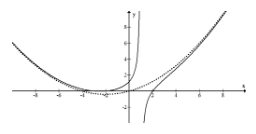
Sometimes a function will have an asymptote that does not look like a line. Take a look at the following function:
\(f(x)=\frac{\left(x^{2}-4\right)(x+3)}{10(x-1)}\)
The degree of the numerator is 3 while the degree of the denominator is 1 so the slant asymptote will not be a line. However when the graph is observed, there is still a clear pattern as to how this function increases without bound as \(x\) approaches very large and very small numbers.
\(f(x)=\frac{1}{10}\left(x^{2}+4 x\right)-\frac{12}{10(x-1)}\)
As you can see, this looks like a parabola with a remainder. This rational function has a parabola backbone. A backbone is a function that a graph tends towards. This is not technically an oblique asymptote because it is not a line.

Examples
Earlier, you were asked what happens when the power of the numerator exceeds the power of the denominator by more than one. As seen above, when the power of numerator exceeds the power of the denominator by more than one, the function develops a backbone that be shaped like any polynomial. Oblique asymptotes are always lines.
Find the asymptotes and intercepts of the function:
\(f(x)=\frac{x^{3}}{x^{2}-4}\)
The function has vertical asymptotes at \(x=\pm 2\).
After long division, the function becomes:
\(f(x)=x+\frac{4}{x^{2}-4}\)
This makes the oblique asymptote at \(y=x\)
Identify the vertical and oblique asymptotes of the following rational function.
\[
f(x)=\frac{x^{3}-x^{2}-x-1}{(x-3)(x+4)}
\]
After using polynomial long division and rewriting the function with a remainder and non-remainder portion it looks like this:
\[
f(x)=x-2+\frac{13 x-25}{x^{2}+x-12}=x-2+\frac{13 x-25}{(x-3)(x+4)}
\]
The oblique asymptote is \(y=x-2\). The vertical asymptotes are at \(x=3\) and \(x=-4\) which are easier to observe in last form of the function because they clearly don't cancel to become holes.
Create a function with an oblique asymptote at \(y=3 x-1,\) vertical asymptotes at \(x=2,-4\) and includes a hole where \(x\) is 7 .
While there are an infinite number of functions that match these criteria, one example is:
\[
f(x)=3 x-1+\frac{(x-7)}{(x-2)(x+4)(x-7)}
\]
Identify the backbone of the following function and explain why the function does not have an oblique asymptote.
\[
f(x)=\frac{5 x^{5}+27}{x^{3}}
\]
While polynomial long division is possible, it is also possible to just divide each term by \(x^{3}\).
\[
f(x)=\frac{5 x^{5}+27}{x^{3}}=\frac{5 x^{5}}{x^{3}}+\frac{27}{x^{3}}=5 x^{2}+\frac{27}{x^{3}}
\]
The backbone of this function is the parabola \(y=5 x^{2}\). This is not an oblique asymptote because it is not a line.
Review
1. What is an oblique asymptote?
2. How can you tell by looking at the equation of a function if it will have an oblique asymptote or not?
3. Can a function have both an oblique asymptote and a horizontal asymptote? Explain.
For each of the following graphs, sketch the graph and then sketch in the oblique asymptote if it exists. If it doesn’t exist, explain why not.
4.
5.
6.
7.
8.
Find the equation of the oblique asymptote for each of the following rational functions. If there is not an oblique asymptote, explain why not and give an equation of the backbone of the function if one exists.
9. \(f(x)=\frac{x^{3}-7 x-6}{x^{2}-2 x-15}\)
10. \(g(x)=\frac{x^{3}-7 x-6}{x^{4}-3 x^{2}-10}\)
11. \(h(x)=\frac{x^{2}+5 x+6}{x^{2}+2 x+1}\)
12. \(k(x)=\frac{x^{4}+9 x^{3}+21 x^{2}-x-30}{x^{2}+2 x+1}\)
13. Create a function with an oblique asymptotes at \(y=2 x-1,\) a vertical asymptote at \(x=3\) and a hole where \(x\) is 7 .
14. Create a function with an oblique asymptote at \(y=x\), vertical asymptotes at \(x=1,-3\) and no holes.
15. Does a parabola have an oblique asymptote? What about a cubic function?


