
3.7: Logistic Functions
- Page ID
- 13685
\( \newcommand{\vecs}[1]{\overset { \scriptstyle \rightharpoonup} {\mathbf{#1}} } \)
\( \newcommand{\vecd}[1]{\overset{-\!-\!\rightharpoonup}{\vphantom{a}\smash {#1}}} \)
\( \newcommand{\dsum}{\displaystyle\sum\limits} \)
\( \newcommand{\dint}{\displaystyle\int\limits} \)
\( \newcommand{\dlim}{\displaystyle\lim\limits} \)
\( \newcommand{\id}{\mathrm{id}}\) \( \newcommand{\Span}{\mathrm{span}}\)
( \newcommand{\kernel}{\mathrm{null}\,}\) \( \newcommand{\range}{\mathrm{range}\,}\)
\( \newcommand{\RealPart}{\mathrm{Re}}\) \( \newcommand{\ImaginaryPart}{\mathrm{Im}}\)
\( \newcommand{\Argument}{\mathrm{Arg}}\) \( \newcommand{\norm}[1]{\| #1 \|}\)
\( \newcommand{\inner}[2]{\langle #1, #2 \rangle}\)
\( \newcommand{\Span}{\mathrm{span}}\)
\( \newcommand{\id}{\mathrm{id}}\)
\( \newcommand{\Span}{\mathrm{span}}\)
\( \newcommand{\kernel}{\mathrm{null}\,}\)
\( \newcommand{\range}{\mathrm{range}\,}\)
\( \newcommand{\RealPart}{\mathrm{Re}}\)
\( \newcommand{\ImaginaryPart}{\mathrm{Im}}\)
\( \newcommand{\Argument}{\mathrm{Arg}}\)
\( \newcommand{\norm}[1]{\| #1 \|}\)
\( \newcommand{\inner}[2]{\langle #1, #2 \rangle}\)
\( \newcommand{\Span}{\mathrm{span}}\) \( \newcommand{\AA}{\unicode[.8,0]{x212B}}\)
\( \newcommand{\vectorA}[1]{\vec{#1}} % arrow\)
\( \newcommand{\vectorAt}[1]{\vec{\text{#1}}} % arrow\)
\( \newcommand{\vectorB}[1]{\overset { \scriptstyle \rightharpoonup} {\mathbf{#1}} } \)
\( \newcommand{\vectorC}[1]{\textbf{#1}} \)
\( \newcommand{\vectorD}[1]{\overrightarrow{#1}} \)
\( \newcommand{\vectorDt}[1]{\overrightarrow{\text{#1}}} \)
\( \newcommand{\vectE}[1]{\overset{-\!-\!\rightharpoonup}{\vphantom{a}\smash{\mathbf {#1}}}} \)
\( \newcommand{\vecs}[1]{\overset { \scriptstyle \rightharpoonup} {\mathbf{#1}} } \)
\(\newcommand{\longvect}{\overrightarrow}\)
\( \newcommand{\vecd}[1]{\overset{-\!-\!\rightharpoonup}{\vphantom{a}\smash {#1}}} \)
\(\newcommand{\avec}{\mathbf a}\) \(\newcommand{\bvec}{\mathbf b}\) \(\newcommand{\cvec}{\mathbf c}\) \(\newcommand{\dvec}{\mathbf d}\) \(\newcommand{\dtil}{\widetilde{\mathbf d}}\) \(\newcommand{\evec}{\mathbf e}\) \(\newcommand{\fvec}{\mathbf f}\) \(\newcommand{\nvec}{\mathbf n}\) \(\newcommand{\pvec}{\mathbf p}\) \(\newcommand{\qvec}{\mathbf q}\) \(\newcommand{\svec}{\mathbf s}\) \(\newcommand{\tvec}{\mathbf t}\) \(\newcommand{\uvec}{\mathbf u}\) \(\newcommand{\vvec}{\mathbf v}\) \(\newcommand{\wvec}{\mathbf w}\) \(\newcommand{\xvec}{\mathbf x}\) \(\newcommand{\yvec}{\mathbf y}\) \(\newcommand{\zvec}{\mathbf z}\) \(\newcommand{\rvec}{\mathbf r}\) \(\newcommand{\mvec}{\mathbf m}\) \(\newcommand{\zerovec}{\mathbf 0}\) \(\newcommand{\onevec}{\mathbf 1}\) \(\newcommand{\real}{\mathbb R}\) \(\newcommand{\twovec}[2]{\left[\begin{array}{r}#1 \\ #2 \end{array}\right]}\) \(\newcommand{\ctwovec}[2]{\left[\begin{array}{c}#1 \\ #2 \end{array}\right]}\) \(\newcommand{\threevec}[3]{\left[\begin{array}{r}#1 \\ #2 \\ #3 \end{array}\right]}\) \(\newcommand{\cthreevec}[3]{\left[\begin{array}{c}#1 \\ #2 \\ #3 \end{array}\right]}\) \(\newcommand{\fourvec}[4]{\left[\begin{array}{r}#1 \\ #2 \\ #3 \\ #4 \end{array}\right]}\) \(\newcommand{\cfourvec}[4]{\left[\begin{array}{c}#1 \\ #2 \\ #3 \\ #4 \end{array}\right]}\) \(\newcommand{\fivevec}[5]{\left[\begin{array}{r}#1 \\ #2 \\ #3 \\ #4 \\ #5 \\ \end{array}\right]}\) \(\newcommand{\cfivevec}[5]{\left[\begin{array}{c}#1 \\ #2 \\ #3 \\ #4 \\ #5 \\ \end{array}\right]}\) \(\newcommand{\mattwo}[4]{\left[\begin{array}{rr}#1 \amp #2 \\ #3 \amp #4 \\ \end{array}\right]}\) \(\newcommand{\laspan}[1]{\text{Span}\{#1\}}\) \(\newcommand{\bcal}{\cal B}\) \(\newcommand{\ccal}{\cal C}\) \(\newcommand{\scal}{\cal S}\) \(\newcommand{\wcal}{\cal W}\) \(\newcommand{\ecal}{\cal E}\) \(\newcommand{\coords}[2]{\left\{#1\right\}_{#2}}\) \(\newcommand{\gray}[1]{\color{gray}{#1}}\) \(\newcommand{\lgray}[1]{\color{lightgray}{#1}}\) \(\newcommand{\rank}{\operatorname{rank}}\) \(\newcommand{\row}{\text{Row}}\) \(\newcommand{\col}{\text{Col}}\) \(\renewcommand{\row}{\text{Row}}\) \(\newcommand{\nul}{\text{Nul}}\) \(\newcommand{\var}{\text{Var}}\) \(\newcommand{\corr}{\text{corr}}\) \(\newcommand{\len}[1]{\left|#1\right|}\) \(\newcommand{\bbar}{\overline{\bvec}}\) \(\newcommand{\bhat}{\widehat{\bvec}}\) \(\newcommand{\bperp}{\bvec^\perp}\) \(\newcommand{\xhat}{\widehat{\xvec}}\) \(\newcommand{\vhat}{\widehat{\vvec}}\) \(\newcommand{\uhat}{\widehat{\uvec}}\) \(\newcommand{\what}{\widehat{\wvec}}\) \(\newcommand{\Sighat}{\widehat{\Sigma}}\) \(\newcommand{\lt}{<}\) \(\newcommand{\gt}{>}\) \(\newcommand{\amp}{&}\) \(\definecolor{fillinmathshade}{gray}{0.9}\)Exponential growth increases without bound. This is reasonable for some situations; however, for populations there is usually some type of upper bound. This can be caused by limitations on food, space or other scarce resources. The effect of this limiting upper bound is a curve that grows exponentially at first and then slows down and hardly grows at all. This type of growth is called logistic growth. What are some other situations in which logistic growth would be an appropriate model?
Logistic Functions
Logistic growth can be described with a logistic equation. The logistic equation is of the form: \(f(x)=\frac{c}{1+a \cdot b^{x}}\)
The letters \(a, b\) and \(c\) are constants that can be changed to match the situation being modeled. You will have to solve for \(a\) and \(b\) with the information that is given to you in each problem. The constant \(c\) is particularly important because it is the limit to growth. This is also known as the carrying capacity.
The following logistic function has a carrying capacity of 2 which can be directly observed from its graph.
\(f(x)=\frac{2}{1+0.1^{x}}\)
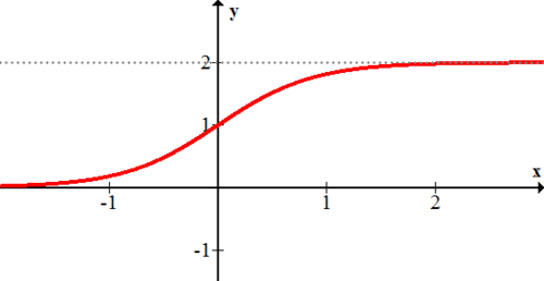
An important note about the logistic function is that it has an inflection point. From the previous graph you can observe that at the point (0,1) the graph transitions from curving up (concave up) to curving down (concave down). This change in curvature will be studied more in calculus, but for now it is important to know that the inflection point occurs halfway between the carrying capacity and the \(x\) axis.
Examples
Earlier, you were asked what situations the logistic model is appropriate for. The logistic model is appropriate whenever the total count has an upper limit and the initial growth is exponential. Examples are the spread of rumors and disease in a limited population and the growth of bacteria or human population when resources are limited.
A rumor is spreading at a school that has a total student population of 1200. Four people know the rumor when it starts and three days later three hundred people know the rumor. About how many people at the school know the rumor by the fourth day?
In a limited population, the count of people who know a rumor is an example of a situation that can be modeled using the logistic function. The population is 1200 so this will be the carrying capacity.
Identifying information: \(c=1200 ;(0,4) ;(3,300)\). First, use the point (0,4) to solve for \(a\).
\(\begin{aligned} \frac{1200}{1+a \cdot b^{0}} &=4 \\ \frac{1200}{1+a} &=4 \\ \frac{1200}{4} &=1+a \\ a &=299 \end{aligned}\)
Next, use the point (3,300) to solve for \(b\).
\(\begin{aligned} \frac{1200}{1+299 \cdot b^{3}} &=300 \\ 4 &=1+299 b^{3} \\ \frac{3}{299} &=b^{3} \\ 0.21568 & \approx b \end{aligned}\)
The modeling equation at \(x=4\) :
\(f(x)=\frac{1200}{1+299 \cdot 0.21568^{x}} \rightarrow f(4) \approx 729\) people
A similar growth pattern will exist with any kind of infectious disease that spreads quickly and can only infect a person or animal once.
A special kind of algae is grown in giant clear plastic tanks and can be harvested to make biofuel. The algae are given plenty of food, water and sunlight to grow rapidly and the only limiting resource is space in the tank. The algae are harvested when 95% of the tank is full leaving the tank 5% full of algae to reproduce and refill the tank. Currently the time between harvests is twenty days and the payoff is 90% harvest. Would you recommend a more optimal harvest schedule?
Identify known quantities and model the growth of the algae.
Known quantities: (0,0.05)\(;(20,0.95) ; c=1\) or \(100 \%\)
\(\begin{aligned} 0.05 &=\frac{1}{1+a \cdot b^{0}} \\ 1+a &=\frac{1}{0.05} \\ a &=19 \\ 0.95 &=\frac{1}{1+19 \cdot b^{20}} \\ 1+19 \cdot b^{20} &=\frac{1}{0.95} \\ b^{20} &=\frac{\left(\frac{1}{0.95}-1\right)}{19} \\ b & \approx 0.74495 \end{aligned}\)
The model for the algae growth is:
\(f(x)=\frac{1}{1+19 \cdot(0.74495)^{x}}\)
The question asks about optimal harvest schedule. Currently the harvest is 90% per 20 day or a unit rate of 4.5% per day. If you shorten the time between harvests where the algae are growing the most efficiently, then potentially this unit rate might be higher. Suppose you leave 15% of the algae in the tank and harvest when it reaches 85%. How much time will that take to yield 70%?
\(\begin{aligned} 0.15 &=\frac{1}{1+19 \cdot(0.74495)^{x}} \\ x_{1} & \approx 4.10897 \\ 0.85 &=\frac{1}{1+19 \cdot(0.74495)^{x}} \\ x_{2} & \approx 15.8914 \end{aligned}\)
\(x_{2}-x_{1} \approx 15.8914-4.10897 \approx 11.78\)
It takes about 12 days for the batches to yield 70% harvest which is a unit rate of about 6% per day. This is a significant increase in efficiency. A harvest schedule that maximizes the time where the logistic curve is steepest creates the fastest overall algae growth.
Determine the logistic model given \(c=12\) and the points (0,9) and (1,11)
The two points give two equations, and the logistic model has two variables. Use these points to solve for \(a\) and \(b\).
\(\begin{aligned} 9 &=\frac{12}{1+a \cdot b^{0}} \\ 1+a &=\frac{12}{9} \\ a &=\frac{1}{3} \\ 11 &=\frac{12}{1+\left(\frac{1}{3}\right) \cdot b^{1}} \\ 1+\left(\frac{1}{3}\right) \cdot b &=\frac{12}{11} \\ b &=0 . \overline{27}=\frac{3}{11} \end{aligned}\)
Thus the approximate model is:
\(f(x)=\frac{12}{1+\left(\frac{1}{3}\right) \cdot\left(\frac{3}{11}\right)^{x}}\)
Determine the logistic model given \(c=7\) and the points (0,2) and (3,5)
The two points give two equations, and the logistic model has two variables. Use these two points to
solve for \(a\) and \(b\).
\(\begin{aligned} 2 &=\frac{7}{1+a} \\ 1+a &=\frac{7}{2} \\ a &=2.5 \\ 5 &=\frac{7}{1+(2.5) \cdot b^{3}} \\ 1+(2.5) \cdot b^{3} &=\frac{7}{5} \\ b^{3} &=0.16 \\ b & \approx 0.5429 \end{aligned}\)
Thus the approximate model is:
\(f(x)=\frac{7}{1+(2.5) \cdot(0.5429)^{x}}\)
Review
For 1-5, determine the logistic model given the carrying capacity and two points.
1. \(c=12 ;(0,5) ;(1,7)\)
2. \(c=200 ;(0,150) ;(5,180)\)
3. \(c=1500 ;(0,150) ;(10,1000)\)
4. \(c=1000000 ;(0,100000) ;(-40,20000)\)
5. \(c=30000000 ;(-60,10000) ;(0,8000000)\)
For \(6-8,\) use the logistic function \(f(x)=\frac{32}{1+3 e^{-x}}\)
6. What is the carrying capacity of the function?
7. What is the \(y\) -intercept of the function?
8. Use your answers to 6 and 7 along with at least two points on the graph to make a sketch of the function.
For \(9-11,\) use the logistic function \(g(x)=\frac{25}{1+4 \cdot 0.2^{x}}\)
9. What is the carrying capacity of the function?
10. What is the \(y\) -intercept of the function?
11. Use your answers to 9 and 10 along with at least two points on the graph to make a sketch of the function.
For \(12-14,\) use the logistic function \(h(x)=\frac{4}{1+2 \cdot 0.68^{x}}\)
12. What is the carrying capacity of the function?
13. What is the \(y\) -intercept of the function?
14. Use your answers to 12 and 13 along with at least two points on the graph to make a sketch of the function.
15. Give an example of a logistic function that is decreasing (models decay). In general, how can you tell from the equation if the logistic function is increasing or decreasing?