
2.4.2: Applications of Histograms
- Page ID
- 5759
\( \newcommand{\vecs}[1]{\overset { \scriptstyle \rightharpoonup} {\mathbf{#1}} } \)
\( \newcommand{\vecd}[1]{\overset{-\!-\!\rightharpoonup}{\vphantom{a}\smash {#1}}} \)
\( \newcommand{\id}{\mathrm{id}}\) \( \newcommand{\Span}{\mathrm{span}}\)
( \newcommand{\kernel}{\mathrm{null}\,}\) \( \newcommand{\range}{\mathrm{range}\,}\)
\( \newcommand{\RealPart}{\mathrm{Re}}\) \( \newcommand{\ImaginaryPart}{\mathrm{Im}}\)
\( \newcommand{\Argument}{\mathrm{Arg}}\) \( \newcommand{\norm}[1]{\| #1 \|}\)
\( \newcommand{\inner}[2]{\langle #1, #2 \rangle}\)
\( \newcommand{\Span}{\mathrm{span}}\)
\( \newcommand{\id}{\mathrm{id}}\)
\( \newcommand{\Span}{\mathrm{span}}\)
\( \newcommand{\kernel}{\mathrm{null}\,}\)
\( \newcommand{\range}{\mathrm{range}\,}\)
\( \newcommand{\RealPart}{\mathrm{Re}}\)
\( \newcommand{\ImaginaryPart}{\mathrm{Im}}\)
\( \newcommand{\Argument}{\mathrm{Arg}}\)
\( \newcommand{\norm}[1]{\| #1 \|}\)
\( \newcommand{\inner}[2]{\langle #1, #2 \rangle}\)
\( \newcommand{\Span}{\mathrm{span}}\) \( \newcommand{\AA}{\unicode[.8,0]{x212B}}\)
\( \newcommand{\vectorA}[1]{\vec{#1}} % arrow\)
\( \newcommand{\vectorAt}[1]{\vec{\text{#1}}} % arrow\)
\( \newcommand{\vectorB}[1]{\overset { \scriptstyle \rightharpoonup} {\mathbf{#1}} } \)
\( \newcommand{\vectorC}[1]{\textbf{#1}} \)
\( \newcommand{\vectorD}[1]{\overrightarrow{#1}} \)
\( \newcommand{\vectorDt}[1]{\overrightarrow{\text{#1}}} \)
\( \newcommand{\vectE}[1]{\overset{-\!-\!\rightharpoonup}{\vphantom{a}\smash{\mathbf {#1}}}} \)
\( \newcommand{\vecs}[1]{\overset { \scriptstyle \rightharpoonup} {\mathbf{#1}} } \)
\( \newcommand{\vecd}[1]{\overset{-\!-\!\rightharpoonup}{\vphantom{a}\smash {#1}}} \)
\(\newcommand{\avec}{\mathbf a}\) \(\newcommand{\bvec}{\mathbf b}\) \(\newcommand{\cvec}{\mathbf c}\) \(\newcommand{\dvec}{\mathbf d}\) \(\newcommand{\dtil}{\widetilde{\mathbf d}}\) \(\newcommand{\evec}{\mathbf e}\) \(\newcommand{\fvec}{\mathbf f}\) \(\newcommand{\nvec}{\mathbf n}\) \(\newcommand{\pvec}{\mathbf p}\) \(\newcommand{\qvec}{\mathbf q}\) \(\newcommand{\svec}{\mathbf s}\) \(\newcommand{\tvec}{\mathbf t}\) \(\newcommand{\uvec}{\mathbf u}\) \(\newcommand{\vvec}{\mathbf v}\) \(\newcommand{\wvec}{\mathbf w}\) \(\newcommand{\xvec}{\mathbf x}\) \(\newcommand{\yvec}{\mathbf y}\) \(\newcommand{\zvec}{\mathbf z}\) \(\newcommand{\rvec}{\mathbf r}\) \(\newcommand{\mvec}{\mathbf m}\) \(\newcommand{\zerovec}{\mathbf 0}\) \(\newcommand{\onevec}{\mathbf 1}\) \(\newcommand{\real}{\mathbb R}\) \(\newcommand{\twovec}[2]{\left[\begin{array}{r}#1 \\ #2 \end{array}\right]}\) \(\newcommand{\ctwovec}[2]{\left[\begin{array}{c}#1 \\ #2 \end{array}\right]}\) \(\newcommand{\threevec}[3]{\left[\begin{array}{r}#1 \\ #2 \\ #3 \end{array}\right]}\) \(\newcommand{\cthreevec}[3]{\left[\begin{array}{c}#1 \\ #2 \\ #3 \end{array}\right]}\) \(\newcommand{\fourvec}[4]{\left[\begin{array}{r}#1 \\ #2 \\ #3 \\ #4 \end{array}\right]}\) \(\newcommand{\cfourvec}[4]{\left[\begin{array}{c}#1 \\ #2 \\ #3 \\ #4 \end{array}\right]}\) \(\newcommand{\fivevec}[5]{\left[\begin{array}{r}#1 \\ #2 \\ #3 \\ #4 \\ #5 \\ \end{array}\right]}\) \(\newcommand{\cfivevec}[5]{\left[\begin{array}{c}#1 \\ #2 \\ #3 \\ #4 \\ #5 \\ \end{array}\right]}\) \(\newcommand{\mattwo}[4]{\left[\begin{array}{rr}#1 \amp #2 \\ #3 \amp #4 \\ \end{array}\right]}\) \(\newcommand{\laspan}[1]{\text{Span}\{#1\}}\) \(\newcommand{\bcal}{\cal B}\) \(\newcommand{\ccal}{\cal C}\) \(\newcommand{\scal}{\cal S}\) \(\newcommand{\wcal}{\cal W}\) \(\newcommand{\ecal}{\cal E}\) \(\newcommand{\coords}[2]{\left\{#1\right\}_{#2}}\) \(\newcommand{\gray}[1]{\color{gray}{#1}}\) \(\newcommand{\lgray}[1]{\color{lightgray}{#1}}\) \(\newcommand{\rank}{\operatorname{rank}}\) \(\newcommand{\row}{\text{Row}}\) \(\newcommand{\col}{\text{Col}}\) \(\renewcommand{\row}{\text{Row}}\) \(\newcommand{\nul}{\text{Nul}}\) \(\newcommand{\var}{\text{Var}}\) \(\newcommand{\corr}{\text{corr}}\) \(\newcommand{\len}[1]{\left|#1\right|}\) \(\newcommand{\bbar}{\overline{\bvec}}\) \(\newcommand{\bhat}{\widehat{\bvec}}\) \(\newcommand{\bperp}{\bvec^\perp}\) \(\newcommand{\xhat}{\widehat{\xvec}}\) \(\newcommand{\vhat}{\widehat{\vvec}}\) \(\newcommand{\uhat}{\widehat{\uvec}}\) \(\newcommand{\what}{\widehat{\wvec}}\) \(\newcommand{\Sighat}{\widehat{\Sigma}}\) \(\newcommand{\lt}{<}\) \(\newcommand{\gt}{>}\) \(\newcommand{\amp}{&}\) \(\definecolor{fillinmathshade}{gray}{0.9}\)Applications of Histograms
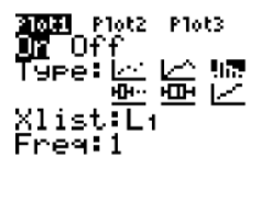
Technology can also be used to plot a histogram. The TI-83 can be used to create a histogram by using STAT and STAT PLOT on the calculator. The TRACE feature can then be used to find the number of values for each bin, and then a frequency distribution table can be constructed from these values. When constructing a histogram using a TI-83 calculator, it's important that your settings are correct on the WINDOW screen. The setting that determines the bin size is the Xscl setting, so you'll want to make sure that the number for Xscl is correct before creating your histogram.
Real-World Application: Piglets
Scientists have invented a new dietary supplement that is supposed to increase the weight of a piglet within its first 3 months of growth. Farmer John fed this supplement to his stock of piglets, and at the end of 3 months, he recorded the weights of 50 randomly selected piglets.
The following table is the recorded weights (in pounds) of the 50 selected piglets:
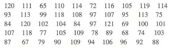
Using the above data set and your calculator, construct a histogram to represent the data. Use a bin size of 10.
The histogram can be created as follows:
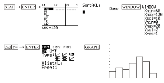
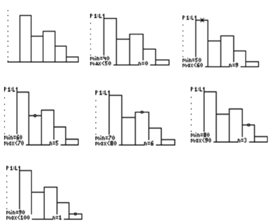
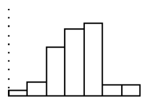
The TRACE Feature
Use the TRACE feature to get information about the data in each bar of the histogram that you created in the previous examples.
First, press
The TRACE feature tells you that in the first bin, which is [60-70), there are 4 values.
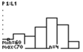
The TRACE feature tells you that in the second bin, which is [70-80), there are 6 values.
To advance to the next bin, or bar, of the histogram, use the cursor and move to the right. The numbers of values for the subsequent bins are 5, 9, 13, 10, and 3, respectively. The information obtained by using the TRACE feature will enable you to create a frequency table and to draw the histogram on paper.
Displaying Data in a Histogram and Constructing a Frequency Distribution Table
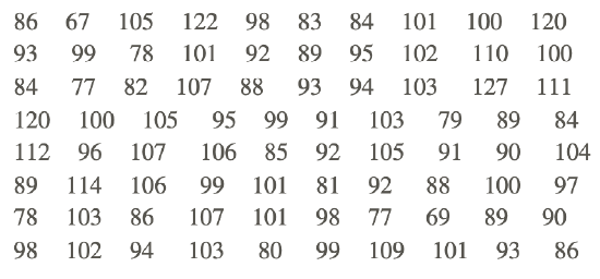
The following data represents the results of a test taken by a group of students:
955670835966885250776980547568785164556774577353
Display the results in a histogram using technology and construct a frequency distribution table using a bin size of 10.
The histogram and the numbers of values for the bins are as shown below:
Now the frequency distribution table can be constructed as follows:
| Bin | Frequency |
|---|---|
| [40−50) | 0 |
| [50−60) | 9 |
| [60−70) | 5 |
| [70−80) | 6 |
| [80−90) | 3 |
| [90−100) |
1 |
Example
Example 1
The following table is the the number of minutes spent practicing per day by a professional violinist for each of the last 80 days:
Display the results in a histogram using technology and construct a frequency distribution table using a bin size of 10.
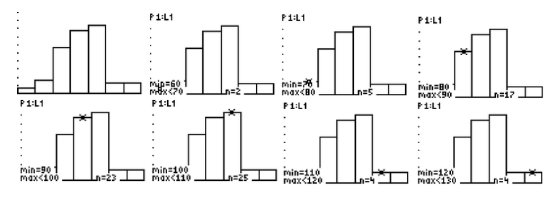
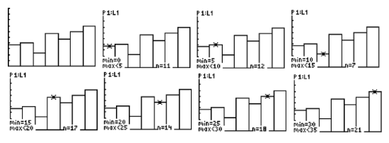
First, press STAT, choose Edit on the EDIT menu, and enter the data values into L1. Since there are so many data values, it's a good idea to then use 1-Var Stats to find the minimum and the maximum data values so that the correct settings for the histogram can be entered in the WINDOW screen. To access 1-Var Stats, after returning to the main screen, press STAT and choose 1-Var Stats on the CALC menu. After pressing ENTER to choose 1-Var Stats, press ENTER again, and then use the down arrow to find the minimum and maximum values. You should see the following:
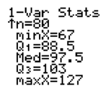
Now that we know that the minimum value is 67 and the maximum value is 127, we can enter the settings for the histogram in the WINDOW screen. To do this, press WINDOW and enter what is shown below:
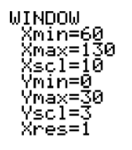
We are now ready to create our histogram. To do so, press 2ND > Y= > ENTER, and make sure you have the following settings:
Finally, press GRAPH, and you should see the histogram shown below:
At this point, you can use the TRACE feature to find the number of values for each bin. Just press TRACE and use the right arrow to move across the screen.
USGS - http://earthquake.usgs.gov/earthquakes/eqarchives/year/graphs.php - CC BY-NC
The numbers for the bins should be 2, 5, 17, 23, 25, 4, and 4, respectively. Notice that 2+5+17+23+25+4+4=80, which is the number of days for which the data exists. Since we now have the frequency for each bin, the frequency distribution table can be created as follows:
| Bin | Frequency |
|---|---|
| [60−70) | 2 |
| [70−80) | 5 |
| [80−90) | 17 |
| [90−100) | 23 |
| [100−110) | 25 |
| [110−120) | 4 |
| [120−130) | 4 |
Review
Use the histogram shown below to answer the following questions:
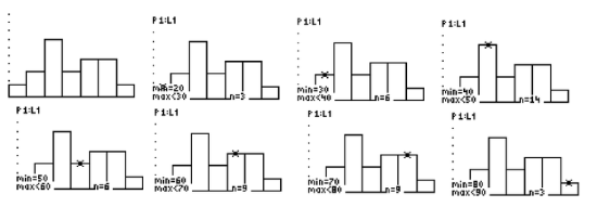
- What is the bin size for the histogram?
- Which bin(s) have the highest frequency?
- Which bin(s) have the lowest frequency?
- What is the total number of data values represented by the histogram?
- What percentage of the data values are in the bin [60-70)?
Use the histogram shown below to answer the following questions
- What is the bin size for the histogram?
- Which bin(s) have the highest frequency?
- Which bin(s) have the lowest frequency?
- What is the total number of data values represented by the histogram?
- What percentage of the data values are in the bin [15-20)?
Vocabulary
| Term | Definition |
|---|---|
| trace feature | The trace feature is a feature on the TI calculator that gives individual values to the five number summary of the box-and-whisker plot. |
Additional Resources
Video: Applications of Histograms Principles
Activities: Applications of Histograms Discussion Questions
Lesson Plans: Creating Histograms with Technology Lesson Plan
Practice: Applications of Histograms
Real World: Steam and Leaf Plots - Gaming Statistics