2.8.1: Understand and Create Stem and Leaf Plots
- Page ID
- 5774
\( \newcommand{\vecs}[1]{\overset { \scriptstyle \rightharpoonup} {\mathbf{#1}} } \)
\( \newcommand{\vecd}[1]{\overset{-\!-\!\rightharpoonup}{\vphantom{a}\smash {#1}}} \)
\( \newcommand{\id}{\mathrm{id}}\) \( \newcommand{\Span}{\mathrm{span}}\)
( \newcommand{\kernel}{\mathrm{null}\,}\) \( \newcommand{\range}{\mathrm{range}\,}\)
\( \newcommand{\RealPart}{\mathrm{Re}}\) \( \newcommand{\ImaginaryPart}{\mathrm{Im}}\)
\( \newcommand{\Argument}{\mathrm{Arg}}\) \( \newcommand{\norm}[1]{\| #1 \|}\)
\( \newcommand{\inner}[2]{\langle #1, #2 \rangle}\)
\( \newcommand{\Span}{\mathrm{span}}\)
\( \newcommand{\id}{\mathrm{id}}\)
\( \newcommand{\Span}{\mathrm{span}}\)
\( \newcommand{\kernel}{\mathrm{null}\,}\)
\( \newcommand{\range}{\mathrm{range}\,}\)
\( \newcommand{\RealPart}{\mathrm{Re}}\)
\( \newcommand{\ImaginaryPart}{\mathrm{Im}}\)
\( \newcommand{\Argument}{\mathrm{Arg}}\)
\( \newcommand{\norm}[1]{\| #1 \|}\)
\( \newcommand{\inner}[2]{\langle #1, #2 \rangle}\)
\( \newcommand{\Span}{\mathrm{span}}\) \( \newcommand{\AA}{\unicode[.8,0]{x212B}}\)
\( \newcommand{\vectorA}[1]{\vec{#1}} % arrow\)
\( \newcommand{\vectorAt}[1]{\vec{\text{#1}}} % arrow\)
\( \newcommand{\vectorB}[1]{\overset { \scriptstyle \rightharpoonup} {\mathbf{#1}} } \)
\( \newcommand{\vectorC}[1]{\textbf{#1}} \)
\( \newcommand{\vectorD}[1]{\overrightarrow{#1}} \)
\( \newcommand{\vectorDt}[1]{\overrightarrow{\text{#1}}} \)
\( \newcommand{\vectE}[1]{\overset{-\!-\!\rightharpoonup}{\vphantom{a}\smash{\mathbf {#1}}}} \)
\( \newcommand{\vecs}[1]{\overset { \scriptstyle \rightharpoonup} {\mathbf{#1}} } \)
\( \newcommand{\vecd}[1]{\overset{-\!-\!\rightharpoonup}{\vphantom{a}\smash {#1}}} \)
\(\newcommand{\avec}{\mathbf a}\) \(\newcommand{\bvec}{\mathbf b}\) \(\newcommand{\cvec}{\mathbf c}\) \(\newcommand{\dvec}{\mathbf d}\) \(\newcommand{\dtil}{\widetilde{\mathbf d}}\) \(\newcommand{\evec}{\mathbf e}\) \(\newcommand{\fvec}{\mathbf f}\) \(\newcommand{\nvec}{\mathbf n}\) \(\newcommand{\pvec}{\mathbf p}\) \(\newcommand{\qvec}{\mathbf q}\) \(\newcommand{\svec}{\mathbf s}\) \(\newcommand{\tvec}{\mathbf t}\) \(\newcommand{\uvec}{\mathbf u}\) \(\newcommand{\vvec}{\mathbf v}\) \(\newcommand{\wvec}{\mathbf w}\) \(\newcommand{\xvec}{\mathbf x}\) \(\newcommand{\yvec}{\mathbf y}\) \(\newcommand{\zvec}{\mathbf z}\) \(\newcommand{\rvec}{\mathbf r}\) \(\newcommand{\mvec}{\mathbf m}\) \(\newcommand{\zerovec}{\mathbf 0}\) \(\newcommand{\onevec}{\mathbf 1}\) \(\newcommand{\real}{\mathbb R}\) \(\newcommand{\twovec}[2]{\left[\begin{array}{r}#1 \\ #2 \end{array}\right]}\) \(\newcommand{\ctwovec}[2]{\left[\begin{array}{c}#1 \\ #2 \end{array}\right]}\) \(\newcommand{\threevec}[3]{\left[\begin{array}{r}#1 \\ #2 \\ #3 \end{array}\right]}\) \(\newcommand{\cthreevec}[3]{\left[\begin{array}{c}#1 \\ #2 \\ #3 \end{array}\right]}\) \(\newcommand{\fourvec}[4]{\left[\begin{array}{r}#1 \\ #2 \\ #3 \\ #4 \end{array}\right]}\) \(\newcommand{\cfourvec}[4]{\left[\begin{array}{c}#1 \\ #2 \\ #3 \\ #4 \end{array}\right]}\) \(\newcommand{\fivevec}[5]{\left[\begin{array}{r}#1 \\ #2 \\ #3 \\ #4 \\ #5 \\ \end{array}\right]}\) \(\newcommand{\cfivevec}[5]{\left[\begin{array}{c}#1 \\ #2 \\ #3 \\ #4 \\ #5 \\ \end{array}\right]}\) \(\newcommand{\mattwo}[4]{\left[\begin{array}{rr}#1 \amp #2 \\ #3 \amp #4 \\ \end{array}\right]}\) \(\newcommand{\laspan}[1]{\text{Span}\{#1\}}\) \(\newcommand{\bcal}{\cal B}\) \(\newcommand{\ccal}{\cal C}\) \(\newcommand{\scal}{\cal S}\) \(\newcommand{\wcal}{\cal W}\) \(\newcommand{\ecal}{\cal E}\) \(\newcommand{\coords}[2]{\left\{#1\right\}_{#2}}\) \(\newcommand{\gray}[1]{\color{gray}{#1}}\) \(\newcommand{\lgray}[1]{\color{lightgray}{#1}}\) \(\newcommand{\rank}{\operatorname{rank}}\) \(\newcommand{\row}{\text{Row}}\) \(\newcommand{\col}{\text{Col}}\) \(\renewcommand{\row}{\text{Row}}\) \(\newcommand{\nul}{\text{Nul}}\) \(\newcommand{\var}{\text{Var}}\) \(\newcommand{\corr}{\text{corr}}\) \(\newcommand{\len}[1]{\left|#1\right|}\) \(\newcommand{\bbar}{\overline{\bvec}}\) \(\newcommand{\bhat}{\widehat{\bvec}}\) \(\newcommand{\bperp}{\bvec^\perp}\) \(\newcommand{\xhat}{\widehat{\xvec}}\) \(\newcommand{\vhat}{\widehat{\vvec}}\) \(\newcommand{\uhat}{\widehat{\uvec}}\) \(\newcommand{\what}{\widehat{\wvec}}\) \(\newcommand{\Sighat}{\widehat{\Sigma}}\) \(\newcommand{\lt}{<}\) \(\newcommand{\gt}{>}\) \(\newcommand{\amp}{&}\) \(\definecolor{fillinmathshade}{gray}{0.9}\)Stem-and-Leaf Plots
In statistics, data is represented in tables, charts, and graphs. One disadvantage of representing data in these ways is that the actual data values are often not retained. One way to ensure that the data values are kept intact is to graph the values in a stem-and-leaf plot. A stem-and-leaf plot is a method of organizing the data that includes sorting the data and graphing it at the same time. This type of graph uses a stem as the leading part of a data value and a leaf as the remaining part of the value. The result is a graph that displays the sorted data in groups, or classes. A stem-and-leaf plot is used most when the number of data values is large, and it allows you to easily calculate the mode and the median of a data set.
Constructing a Stem-and-Leaf Plot
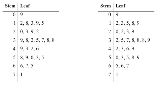
Construct a stem-and-leaf plot for the following data values:

The stem-and-leaf plot can be constructed as follows. We will first create the stem-and-leaf plot, and then we will organize the values of the leaves.
Interpreting Stem-and-Leaf Plots
The following numbers represent the growth (in centimeters) of some plants after 25 days.
Construct a stem-and-leaf plot to represent the data, and list 3 facts that you know about the growth of the plants.
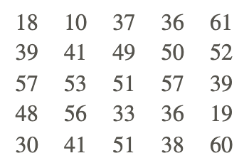
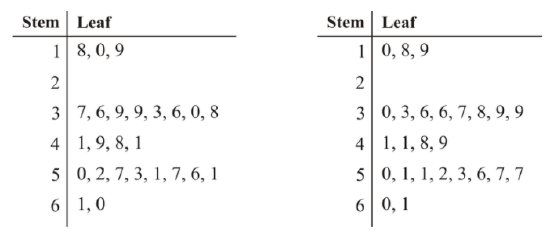
Note that there are no leaves for the second stem. If there are no values in a class, do not enter a value in the leaf−just leave it blank.
As for 3 facts that you know about the growth of the plants, answers will vary, but the following are some possible responses:
- From the stem-and-leaf plot, the growth of the plants ranged from a minimum of 10 cm to a maximum of 61 cm.
- The median of the data set is the value in the 13th position, which is 41 cm.
- There was no growth recorded in the class of 20 cm, so there is no number in the leaf row.
- The data set is multimodal.
Finding the Mode and the Median
The following stem-and-leaf plot represents the ages of 23 people waiting in line at Tim Horton’s. What is the mode and the median of the ages? How many people are older than 32?
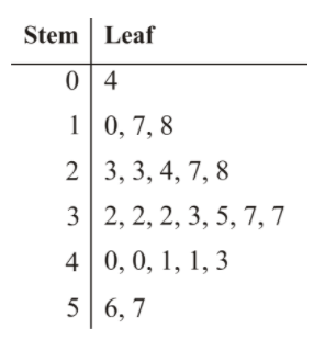
The mode is the value that appears the most often, and here it is 32. As for the median, since there are 23 data values, the median is the value that appears in the 12th position. From the stem-and-leaf plot, it's clear that this value is 32, so the median of the data set is 32 as well. Finally, to find the number of people older than 32, count the number of all the digits after the number 2 in the row that has 3 as its stem. There are a total of 11 digits, so 11 people are older than 32.
Example
At a local veterinarian school, the number of animals treated each day over a period of 20 days was recorded.
Example 1
Construct a stem-and-leaf plot for the data set, which is as follows:

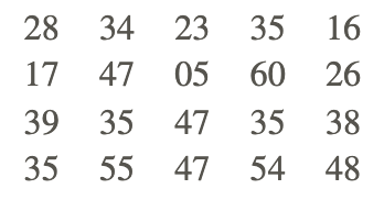
What is the mode and the median of the data set?
Step 1: Create the stem-and-leaf plot.
Some people prefer to arrange the data in order before the stems and leaves are created. This will ensure that the values of the leaves are in order. However, this is not necessary and can take a great deal of time if the data set is large.
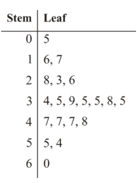
The leading digit of a data value is used as the stem, and the trailing digit is used as the leaf. The numbers in the stem column should be consecutive numbers that begin with the smallest class and continue to the largest class.
Step 2: Organize the values in each leaf row.
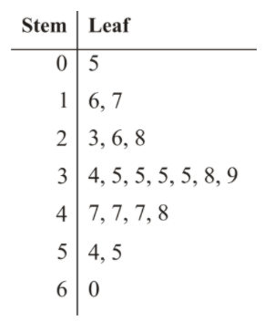
Now that the graph has been constructed, there is a great deal of information that can be learned from it.
The number of values in the leaf column should equal the number of data values that were given in the table. The value that appears the most often in the same leaf row is the trailing digit of the mode of the data set. The mode of this data set is 35. For 7 of the 20 days, the number of animals receiving treatment was between 34 and 39. The veterinarian school treated a minimum of 5 animals and a maximum of 60 animals on any one day. The median of the data can be quickly calculated by using the values in the leaf column to locate the value in the middle position. In this stem and leaf plot, the median is the mean of the sum of the numbers represented by the 10th and the 11th leaves:

Review
- The following stem-and-leaf plot shows the cholesterol levels of a random number of students. These values range from 2.3 to 8.9. What percentage of the students have levels between 5.0 and 7.1,
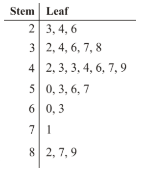
inclusive?
a. 6 %
b. 20%
c. 24%
d. 28%
2. Just like Presidents of the United States, Canadian Prime Ministers must be sworn into office. The following data represents the ages of 22 Canadian Prime Ministers when they were sworn into office. Construct a stem-and-leaf plot to represent the ages, and list 4 facts that you know from the graph.
52 74 60 39 65 46 55 66 54 51 70 47 69 47 57 46 48 66 61 59 46 45
Use the stem-and-leaf plot below to answer the following questions:
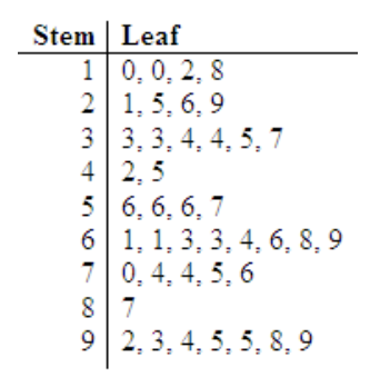
- What is the mode of the data set?
- What is the median of the data set?
- What is the minimum of the data set?
- What is the maximum of the data set?
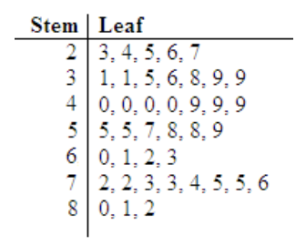
Use the stem-and-leaf plot below to answer the following questions:
Additional Resources
PLIX: Play, Learn, Interact, eXplore - Ordering Leaves
Video: Histograms
Activities: Stem-and-Leaf Plots Discussion Questions - P&S
Study Aids: Presenting Univariate Data
Lesson Plans: Stem and Leaf Plots Lesson Plan
Practice: Understand and Create Stem and Leaf Plots
Real World: Timetable Travel

