
6.1: Normal Distributions
- Page ID
- 5729
\( \newcommand{\vecs}[1]{\overset { \scriptstyle \rightharpoonup} {\mathbf{#1}} } \)
\( \newcommand{\vecd}[1]{\overset{-\!-\!\rightharpoonup}{\vphantom{a}\smash {#1}}} \)
\( \newcommand{\id}{\mathrm{id}}\) \( \newcommand{\Span}{\mathrm{span}}\)
( \newcommand{\kernel}{\mathrm{null}\,}\) \( \newcommand{\range}{\mathrm{range}\,}\)
\( \newcommand{\RealPart}{\mathrm{Re}}\) \( \newcommand{\ImaginaryPart}{\mathrm{Im}}\)
\( \newcommand{\Argument}{\mathrm{Arg}}\) \( \newcommand{\norm}[1]{\| #1 \|}\)
\( \newcommand{\inner}[2]{\langle #1, #2 \rangle}\)
\( \newcommand{\Span}{\mathrm{span}}\)
\( \newcommand{\id}{\mathrm{id}}\)
\( \newcommand{\Span}{\mathrm{span}}\)
\( \newcommand{\kernel}{\mathrm{null}\,}\)
\( \newcommand{\range}{\mathrm{range}\,}\)
\( \newcommand{\RealPart}{\mathrm{Re}}\)
\( \newcommand{\ImaginaryPart}{\mathrm{Im}}\)
\( \newcommand{\Argument}{\mathrm{Arg}}\)
\( \newcommand{\norm}[1]{\| #1 \|}\)
\( \newcommand{\inner}[2]{\langle #1, #2 \rangle}\)
\( \newcommand{\Span}{\mathrm{span}}\) \( \newcommand{\AA}{\unicode[.8,0]{x212B}}\)
\( \newcommand{\vectorA}[1]{\vec{#1}} % arrow\)
\( \newcommand{\vectorAt}[1]{\vec{\text{#1}}} % arrow\)
\( \newcommand{\vectorB}[1]{\overset { \scriptstyle \rightharpoonup} {\mathbf{#1}} } \)
\( \newcommand{\vectorC}[1]{\textbf{#1}} \)
\( \newcommand{\vectorD}[1]{\overrightarrow{#1}} \)
\( \newcommand{\vectorDt}[1]{\overrightarrow{\text{#1}}} \)
\( \newcommand{\vectE}[1]{\overset{-\!-\!\rightharpoonup}{\vphantom{a}\smash{\mathbf {#1}}}} \)
\( \newcommand{\vecs}[1]{\overset { \scriptstyle \rightharpoonup} {\mathbf{#1}} } \)
\( \newcommand{\vecd}[1]{\overset{-\!-\!\rightharpoonup}{\vphantom{a}\smash {#1}}} \)
\(\newcommand{\avec}{\mathbf a}\) \(\newcommand{\bvec}{\mathbf b}\) \(\newcommand{\cvec}{\mathbf c}\) \(\newcommand{\dvec}{\mathbf d}\) \(\newcommand{\dtil}{\widetilde{\mathbf d}}\) \(\newcommand{\evec}{\mathbf e}\) \(\newcommand{\fvec}{\mathbf f}\) \(\newcommand{\nvec}{\mathbf n}\) \(\newcommand{\pvec}{\mathbf p}\) \(\newcommand{\qvec}{\mathbf q}\) \(\newcommand{\svec}{\mathbf s}\) \(\newcommand{\tvec}{\mathbf t}\) \(\newcommand{\uvec}{\mathbf u}\) \(\newcommand{\vvec}{\mathbf v}\) \(\newcommand{\wvec}{\mathbf w}\) \(\newcommand{\xvec}{\mathbf x}\) \(\newcommand{\yvec}{\mathbf y}\) \(\newcommand{\zvec}{\mathbf z}\) \(\newcommand{\rvec}{\mathbf r}\) \(\newcommand{\mvec}{\mathbf m}\) \(\newcommand{\zerovec}{\mathbf 0}\) \(\newcommand{\onevec}{\mathbf 1}\) \(\newcommand{\real}{\mathbb R}\) \(\newcommand{\twovec}[2]{\left[\begin{array}{r}#1 \\ #2 \end{array}\right]}\) \(\newcommand{\ctwovec}[2]{\left[\begin{array}{c}#1 \\ #2 \end{array}\right]}\) \(\newcommand{\threevec}[3]{\left[\begin{array}{r}#1 \\ #2 \\ #3 \end{array}\right]}\) \(\newcommand{\cthreevec}[3]{\left[\begin{array}{c}#1 \\ #2 \\ #3 \end{array}\right]}\) \(\newcommand{\fourvec}[4]{\left[\begin{array}{r}#1 \\ #2 \\ #3 \\ #4 \end{array}\right]}\) \(\newcommand{\cfourvec}[4]{\left[\begin{array}{c}#1 \\ #2 \\ #3 \\ #4 \end{array}\right]}\) \(\newcommand{\fivevec}[5]{\left[\begin{array}{r}#1 \\ #2 \\ #3 \\ #4 \\ #5 \\ \end{array}\right]}\) \(\newcommand{\cfivevec}[5]{\left[\begin{array}{c}#1 \\ #2 \\ #3 \\ #4 \\ #5 \\ \end{array}\right]}\) \(\newcommand{\mattwo}[4]{\left[\begin{array}{rr}#1 \amp #2 \\ #3 \amp #4 \\ \end{array}\right]}\) \(\newcommand{\laspan}[1]{\text{Span}\{#1\}}\) \(\newcommand{\bcal}{\cal B}\) \(\newcommand{\ccal}{\cal C}\) \(\newcommand{\scal}{\cal S}\) \(\newcommand{\wcal}{\cal W}\) \(\newcommand{\ecal}{\cal E}\) \(\newcommand{\coords}[2]{\left\{#1\right\}_{#2}}\) \(\newcommand{\gray}[1]{\color{gray}{#1}}\) \(\newcommand{\lgray}[1]{\color{lightgray}{#1}}\) \(\newcommand{\rank}{\operatorname{rank}}\) \(\newcommand{\row}{\text{Row}}\) \(\newcommand{\col}{\text{Col}}\) \(\renewcommand{\row}{\text{Row}}\) \(\newcommand{\nul}{\text{Nul}}\) \(\newcommand{\var}{\text{Var}}\) \(\newcommand{\corr}{\text{corr}}\) \(\newcommand{\len}[1]{\left|#1\right|}\) \(\newcommand{\bbar}{\overline{\bvec}}\) \(\newcommand{\bhat}{\widehat{\bvec}}\) \(\newcommand{\bperp}{\bvec^\perp}\) \(\newcommand{\xhat}{\widehat{\xvec}}\) \(\newcommand{\vhat}{\widehat{\vvec}}\) \(\newcommand{\uhat}{\widehat{\uvec}}\) \(\newcommand{\what}{\widehat{\wvec}}\) \(\newcommand{\Sighat}{\widehat{\Sigma}}\) \(\newcommand{\lt}{<}\) \(\newcommand{\gt}{>}\) \(\newcommand{\amp}{&}\) \(\definecolor{fillinmathshade}{gray}{0.9}\)Applications of the Normal Distribution
The normal distribution is the foundation for statistical inference and will be an essential part of many of those topics in later chapters. In the meantime, this section will cover some of the types of questions that can be answered using the properties of a normal distribution. The first examples deal with more theoretical questions that will help you master basic understandings and computational skills, while the later problems will provide examples with real data, or at least a real context.
Unknown Value Problems
If you understand the relationship between the area under a density curve and mean, standard deviation, and z-scores, you should be able to solve problems in which you are provided all but one of these values and are asked to calculate the remaining value. In the last lesson, we found the probability that a variable is within a particular range, or the area under a density curve within that range. What if you are asked to find a value that gives a particular probability?
Calculating an Unknown Value
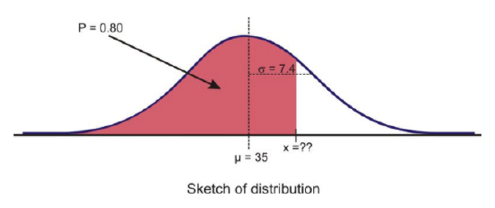
Given the normally-distributed random variable X, with μ=35 and σ=7.4, what is the value of X where the probability of experiencing a value less than it is 80%?
As suggested before, it is important and helpful to sketch the distribution.
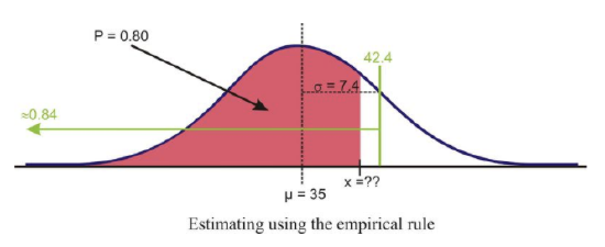
If we had to estimate an actual value first, we know from the Empirical Rule that about 84% of the data is below one standard deviation to the right of the mean.
μ+1σ=35+7.4=42.4
Therefore, we expect the answer to be slightly below this value.
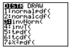
When we were given a value of the variable and were asked to find the percentage or probability, we used a z-table or the 'normalcdf(' command on a graphing calculator. But how do we find a value given the percentage? Again, the table has its limitations in this case, and graphing calculators and computer software are much more convenient and accurate. The command on the TI-83/84 calculator is 'invNorm('. You may have seen it already in the DISTR menu.
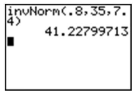
The syntax for this command is as follows:
'InvNorm(percentage or probability to the left, mean, standard deviation)'
Make sure to enter the values in the correct order, such as in the example below:
Unknown Mean or Standard Deviation
Estimating an Unknown Mean
For a normally distributed random variable, σ=4.5, x=20, and p=0.05, Estimate μ.
To solve this problem, first draw a sketch:
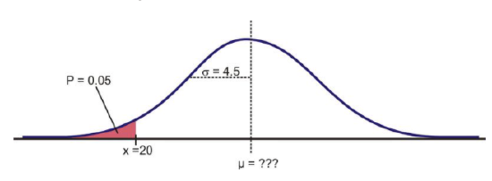
Remember that about 95% of the data is within 2 standard deviations of the mean. This would leave 2.5% of the data in the lower tail, so our 5% value must be less than 9 units from the mean.
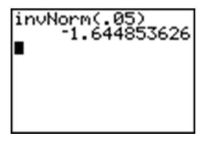
Because we do not know the mean, we have to use the standard normal curve and calculate a z-score using the 'invNorm(' command. The result, −1.645, confirms the prediction that the value is less than 2 standard deviations from the mean.
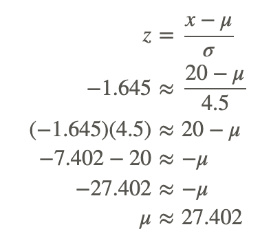
Now, plug in the known quantities into the z-score formula and solve for μ as follows:
Estimating an Unknown Standard Deviation
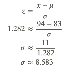
For a normally-distributed random variable, μ=83, x=94, and p=0.90. Find σ.
Again, let’s first look at a sketch of the distribution.
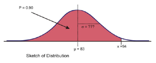
Since about 97.5% of the data is below 2 standard deviations, it seems reasonable to estimate that the x value is less than two standard deviations away from the mean and that σ might be around 7 or 8.
Again, the first step to see if our prediction is right is to use 'invNorm(' to calculate the z-score. Remember that since we are not entering a mean or standard deviation, the result is based on the assumption that μ=0 and σ=1.
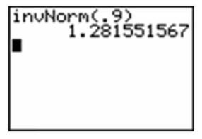
Now, use the z-score formula and solve for σ as follows:
Technology Note: Drawing a Distribution on the TI-83/84 Calculator
The TI-83/84 calculator will draw a distribution for you, but before doing so, we need to set an appropriate window (see screen below) and delete or turn off any functions or plots. Let’s use the last example and draw the shaded region below 94 under a normal curve with μ=83 and σ=8.583. Remember from the Empirical Rule that we probably want to show about 3 standard deviations away from 83 in either direction. If we use 9 as an estimate for σ, then we should open our window 27 units above and below 83. The y settings can be a bit tricky, but with a little practice, you will get used to determining the maximum percentage of area near the mean.
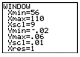
The reason that we went below the x-axis is to leave room for the text, as you will see.
Now, press [2ND][DISTR] and arrow over to the DRAW menu.
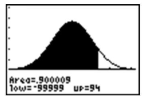
Choose the 'ShadeNorm(' command. With this command, you enter the values just as if you were doing a 'normalcdf(' calculation. The syntax for the 'ShadeNorm(' command is as follows:
'ShadeNorm(lower bound, upper bound, mean, standard deviation)'
Enter the values shown in the following screenshot:

Next, press [ENTER] to see the result. It should appear as follows:
Technology Note: The 'normalpdf(' Command on the TI-83/84 Calculator
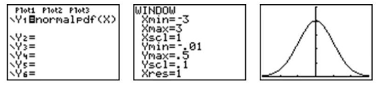
You may have noticed that the first option in the DISTR menu is 'normalpdf(', which stands for a normal probability density function. It is the option you used in lesson 5.1 to draw the graph of a normal distribution. Many students wonder what this function is for and occasionally even use it by mistake to calculate what they think are cumulative probabilities, but this function is actually the mathematical formula for drawing a normal distribution. You can find this formula in the resources at the end of the lesson if you are interested. The numbers this function returns are not really useful to us statistically. The primary purpose for this function is to draw the normal curve.
To do this, first be sure to turn off any plots and clear out any functions. Then press [Y=], insert 'normalpdf(', enter 'X', and close the parentheses as shown. Because we did not specify a mean and standard deviation, the standard normal curve will be drawn. Finally, enter the following window settings, which are necessary to fit most of the curve on the screen (think about the Empirical Rule when deciding on settings), and press [GRAPH]. The normal curve below should appear on your screen.
Normal Distributions with Real Data
The foundation of performing experiments by collecting surveys and samples is most often based on the normal distribution, as you will learn in greater detail in later chapters. Here are two examples to get you started.
Using Technology
The Information Centre of the National Health Service in Britain collects and publishes a great deal of information and statistics on health issues affecting the population. One such comprehensive data set tracks information about the health of children1. According to its statistics, in 2006, the mean height of 12-year-old boys was 152.9 cm, with a standard deviation estimate of approximately 8.5 cm. (These are not the exact figures for the population, and in later chapters, we will learn how they are calculated and how accurate they may be, but for now, we will assume that they are a reasonable estimate of the true parameters.)
If 12-year-old Cecil is 158 cm, approximately what percentage of all 12-year-old boys in Britain is he taller than?
We first must assume that the height of 12-year-old boys in Britain is normally distributed, and this seems like a reasonable assumption to make. As always, draw a sketch and estimate a reasonable answer prior to calculating the percentage. In this case, let’s use the calculator to sketch the distribution and the shading. First decide on an appropriate window that includes about 3 standard deviations on either side of the mean. In this case, 3 standard deviations is about 25.5 cm, so add and subtract this value to/from the mean to find the horizontal extremes. Then enter the appropriate 'ShadeNorm(' command as shown:
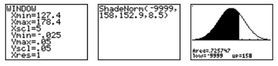
From this data, we would estimate that Cecil is taller than about 73% of 12-year-old boys. We could also phrase our assumption this way: the probability of a randomly selected British 12-year-old boy being shorter than Cecil is about 0.73. Often with data like this, we use percentiles. We would say that Cecil is in the 73rd percentile for height among 12-year-old boys in Britain.
How tall would Cecil need to be in order to be in the top 1% of all 12-year-old boys in Britain?
Here is a sketch:
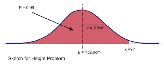
In this case, we are given the percentage, so we need to use the 'invNorm(' command as shown.
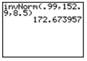
Our results indicate that Cecil would need to be about 173 cm tall to be in the top 1% of 12-year-old boys in Britain.
Example
Example 1
Suppose that the distribution of the masses of female marine iguanas in Puerto Villamil in the Galapagos Islands is approximately normal, with a mean mass of 950 g and a standard deviation of 325 g. There are very few young marine iguanas in the populated areas of the islands, because feral cats tend to kill them. How rare is it that we would find a female marine iguana with a mass less than 400 g in this area?
It helps to draw a picture of the situation:
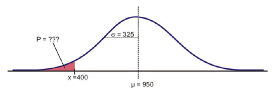
Using a graphing calculator, we can approximate the probability of a female marine iguana being less than 400 grams as follows:
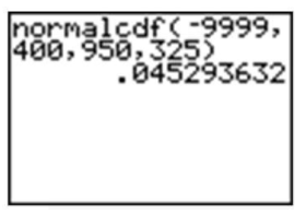
With a probability of approximately 0.045, or only about 5%, we could say it is rather unlikely that we would find an iguana this small.
Review
- Which of the following intervals contains the middle 95% of the data in a standard normal distribution?
a. z<2
b. z≤1.645
c. z≤1.96
d. −1.645≤z≤1.645
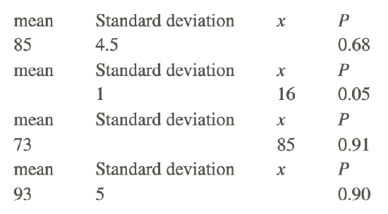
e. −1.96≤z≤1.96 - For each of the following problems, X is a continuous random variable with a normal distribution and the given mean and standard deviation. P is the probability of a value of the distribution being less than x. Find the missing value and sketch and shade the distribution.
- What is the z-score for the lower quartile in a standard normal distribution?
- The manufacturing process at a metal-parts factory produces some slight variation in the diameter of metal ball bearings. The quality control experts claim that the bearings produced have a mean diameter of 1.4 cm. If the diameter is more than 0.0035 cm too wide or too narrow, they will not work properly. In order to maintain its reliable reputation, the company wishes to insure that no more than one-tenth of 1% of the bearings that are defective. What would the standard deviation of the manufactured bearings need to be in order to meet this goal?
- Suppose that the wrapper of a certain candy bar lists its weight as 2.13 ounces. Naturally, the weights of individual bars vary somewhat. Suppose that the weights of these candy bars vary according to a normal distribution, with μ=2.2 ounces and σ=0.04ounces.
a. What proportion of the candy bars weigh less than the advertised weight?
b. What proportion of the candy bars weight between 2.2 and 2.3 ounces?
c. A candy bar of what weight would be heavier than all but 1% of the candy bars out there?
d. If the manufacturer wants to adjust the production process so that no more than 1 candy bar in 1000 weighs less than the advertised weight, what would the mean of the actual weights need to be? (Assume the standard deviation remains the same.)
e. If the manufacturer wants to adjust the production process so that the mean remains at 2.2 ounces and no more than 1 candy bar in 1000 weighs less than the advertised weight, how small does the standard deviation of the weights need to be? - How do the probabilities of a standard normal curve apply to making decisions about unknown parameters for a population given a sample?
References
National Health Services- United Kingdom
The New York Times
- The heights of women are ages 18 to 24 are approximately normally distributed with mean 64.5 inches and standard deviation 2.5 inches.
a. Draw a frequency curve for this distribution.
b. What percent of women in this age group are taller than 62 inches? Taller than 69.5 inches? Shorter than 59.5 inches? - Scores on an intelligence test for the age group 20 to 34 are approximately normally distributed with mean 110 and standard deviation 25. About what percent of people in this age group have scores
a. Above 110?
b. Above 160?
c. Below 85?
d. What percent of people ages 20 – 34 have IQs below 100?
e. What percent of people ages 20 – 34 have IQs 100 or above?
f. What percent of people ages 20 – 34 have IQs above 145?
g. If only 1% of people in this age group have IQs higher than Elizabeth, what is Elizabeth’s IQ? - Mary scores 750 on the mathematics part of the SAT. Scores on the SAT follow the normal distribution with mean 500 and standard deviation 100. John takes the ACT math test. He scores 26. This test has a mean of approximately 18 and standard deviation of 6. The scores on the ACT follow a normal distribution. If both the SAT and the ACT measure the same kind of ability, who has the better score?
- Scores on an intelligence test for the age group 60 – 64 are approximately normally distributed with mean 90 and standard deviation 25.
a. Joan, who is 60 takes the test and scores 120. Express this as a standard score.
b. Joan’s daughter is 30. She takes the intelligence test and scores 135. Use the information in problem 8 to standardize this score.
c. Who scored higher relative to her age group, Joan or Joan’s daughter? - The average height of 18-year old boys is normally distributed with a mean of 180 cm and a standard deviation of 7 cm. Calculate the percentage of 18-year old boys whose heights are:
a. More than 195 cm
b. Between 163 and 195 cm
c. Between 171 and 187 cm. - Heights for high-school age students in the United States have means and standard deviations of approximately 79 inches and 3 inches for males and 65 inches and 2.5 inches for females. Using your height, find the z-score for a high school age student of your sex and height.
- For each of the following find the proportion for each of the following situations. In all cases, assume the population is normally distributed. a. The proportion of SAT scores that fall below 487 for a group with mean of 510 and a standard deviation of 110. b. The proportion of girls with heights below 34 inches for a group with mean height of 31 inches and a standard deviation of 1 inch. c. The proportion of a large class that scored above you on a test where the mean was 70, the standard deviation was 6 and your score was 75.
- Suppose yearly rainfall totals for a city in upstate New York follow a normal distribution, with mean 20 inches and standard deviation of 5 inches. For a randomly selected year, what is the probability that total rainfall will be in each of the following intervals?
- Less than 12 inches
- Greater than 25 inches
- Between 14 and 24 inches
- Greater than 40 inches
- If your score on a test was 85 and the mean of the test was 75 would you be more satisfied if the standard deviation was 5 or 15? Explain.
- Assuming that IQ scores of adults are normally distributed with a mean of 100 and a standard deviation of 15, find the score that separates the top 15% from the others.
- The following is a list of test grades from a statistic semester exam. The teacher wants to use the empirical rule to decide which of these grades he should assign A, B, C, D and F. 79 86 94 63 83 77 75 74 93 68 90 87 87 96 69 93 87 94 94 83 87 80 79 54 86 80 87
- Determine the mean and then which of these test scores are 3 standard deviations away from the mean, 2 standard deviations away from the mean and 1 standard deviation away from the mean.
- Determine the test scores that will qualify for each letter grade.
- Compute the number of students to earn each letter grade on this particular test.
- Was it appropriate for the teacher to use a normal distribution to determine these letter grades? Explain.
- Suppose the grades on a statistics semester exam follow a normal distribution. It is found that 10% of students scored at least 90 and no more than 20% scored less than 35. What proportion of students scored more than 50? 18. Suppose the arm lengths of females are normally distributed with a standard deviation of 4 cm. It is found that 2% of female arm lengths are greater than 72.2 cm. Find the mean of the distribution.
Vocabulary
| Term | Definition |
|---|---|
| invNorm | The 'invNorm' command on the TI-83/84 calculator is used to find a z-score or value of the variable. |
| normalcdf | The 'normalcdf' command on the TI-83/84 calculator allows you to find the percentage of data in-between two values (or the probability of a randomly chosen value being between those values) in a normal distribution, |
| Normpdf | The primary purpose for the "Normpdf" function on the TI-83/84 calculator is to draw the normal curve. |
| ShadeNorm | The 'ShadeNorm' command on the TI-83/84 calculator allows you to show the shaded region of a normal distribution curve on your calculator. |
Additional Resources
PLIX: Play, Learn, Interact, eXplore - The FDA and Food Safety
Video: Normal Distributions Principles
Activities: Normal Distributions Discussion Questions
Study Aids: Normal Distribution Study Guide
Lesson Plans: Normal Distribution Lesson Plan
Practice: Normal Distributions
Real World: Low Pressure