
6.5: Computing Probabilities for the Standard Normal Distribution
- Page ID
- 5733
\( \newcommand{\vecs}[1]{\overset { \scriptstyle \rightharpoonup} {\mathbf{#1}} } \)
\( \newcommand{\vecd}[1]{\overset{-\!-\!\rightharpoonup}{\vphantom{a}\smash {#1}}} \)
\( \newcommand{\id}{\mathrm{id}}\) \( \newcommand{\Span}{\mathrm{span}}\)
( \newcommand{\kernel}{\mathrm{null}\,}\) \( \newcommand{\range}{\mathrm{range}\,}\)
\( \newcommand{\RealPart}{\mathrm{Re}}\) \( \newcommand{\ImaginaryPart}{\mathrm{Im}}\)
\( \newcommand{\Argument}{\mathrm{Arg}}\) \( \newcommand{\norm}[1]{\| #1 \|}\)
\( \newcommand{\inner}[2]{\langle #1, #2 \rangle}\)
\( \newcommand{\Span}{\mathrm{span}}\)
\( \newcommand{\id}{\mathrm{id}}\)
\( \newcommand{\Span}{\mathrm{span}}\)
\( \newcommand{\kernel}{\mathrm{null}\,}\)
\( \newcommand{\range}{\mathrm{range}\,}\)
\( \newcommand{\RealPart}{\mathrm{Re}}\)
\( \newcommand{\ImaginaryPart}{\mathrm{Im}}\)
\( \newcommand{\Argument}{\mathrm{Arg}}\)
\( \newcommand{\norm}[1]{\| #1 \|}\)
\( \newcommand{\inner}[2]{\langle #1, #2 \rangle}\)
\( \newcommand{\Span}{\mathrm{span}}\) \( \newcommand{\AA}{\unicode[.8,0]{x212B}}\)
\( \newcommand{\vectorA}[1]{\vec{#1}} % arrow\)
\( \newcommand{\vectorAt}[1]{\vec{\text{#1}}} % arrow\)
\( \newcommand{\vectorB}[1]{\overset { \scriptstyle \rightharpoonup} {\mathbf{#1}} } \)
\( \newcommand{\vectorC}[1]{\textbf{#1}} \)
\( \newcommand{\vectorD}[1]{\overrightarrow{#1}} \)
\( \newcommand{\vectorDt}[1]{\overrightarrow{\text{#1}}} \)
\( \newcommand{\vectE}[1]{\overset{-\!-\!\rightharpoonup}{\vphantom{a}\smash{\mathbf {#1}}}} \)
\( \newcommand{\vecs}[1]{\overset { \scriptstyle \rightharpoonup} {\mathbf{#1}} } \)
\( \newcommand{\vecd}[1]{\overset{-\!-\!\rightharpoonup}{\vphantom{a}\smash {#1}}} \)
\(\newcommand{\avec}{\mathbf a}\) \(\newcommand{\bvec}{\mathbf b}\) \(\newcommand{\cvec}{\mathbf c}\) \(\newcommand{\dvec}{\mathbf d}\) \(\newcommand{\dtil}{\widetilde{\mathbf d}}\) \(\newcommand{\evec}{\mathbf e}\) \(\newcommand{\fvec}{\mathbf f}\) \(\newcommand{\nvec}{\mathbf n}\) \(\newcommand{\pvec}{\mathbf p}\) \(\newcommand{\qvec}{\mathbf q}\) \(\newcommand{\svec}{\mathbf s}\) \(\newcommand{\tvec}{\mathbf t}\) \(\newcommand{\uvec}{\mathbf u}\) \(\newcommand{\vvec}{\mathbf v}\) \(\newcommand{\wvec}{\mathbf w}\) \(\newcommand{\xvec}{\mathbf x}\) \(\newcommand{\yvec}{\mathbf y}\) \(\newcommand{\zvec}{\mathbf z}\) \(\newcommand{\rvec}{\mathbf r}\) \(\newcommand{\mvec}{\mathbf m}\) \(\newcommand{\zerovec}{\mathbf 0}\) \(\newcommand{\onevec}{\mathbf 1}\) \(\newcommand{\real}{\mathbb R}\) \(\newcommand{\twovec}[2]{\left[\begin{array}{r}#1 \\ #2 \end{array}\right]}\) \(\newcommand{\ctwovec}[2]{\left[\begin{array}{c}#1 \\ #2 \end{array}\right]}\) \(\newcommand{\threevec}[3]{\left[\begin{array}{r}#1 \\ #2 \\ #3 \end{array}\right]}\) \(\newcommand{\cthreevec}[3]{\left[\begin{array}{c}#1 \\ #2 \\ #3 \end{array}\right]}\) \(\newcommand{\fourvec}[4]{\left[\begin{array}{r}#1 \\ #2 \\ #3 \\ #4 \end{array}\right]}\) \(\newcommand{\cfourvec}[4]{\left[\begin{array}{c}#1 \\ #2 \\ #3 \\ #4 \end{array}\right]}\) \(\newcommand{\fivevec}[5]{\left[\begin{array}{r}#1 \\ #2 \\ #3 \\ #4 \\ #5 \\ \end{array}\right]}\) \(\newcommand{\cfivevec}[5]{\left[\begin{array}{c}#1 \\ #2 \\ #3 \\ #4 \\ #5 \\ \end{array}\right]}\) \(\newcommand{\mattwo}[4]{\left[\begin{array}{rr}#1 \amp #2 \\ #3 \amp #4 \\ \end{array}\right]}\) \(\newcommand{\laspan}[1]{\text{Span}\{#1\}}\) \(\newcommand{\bcal}{\cal B}\) \(\newcommand{\ccal}{\cal C}\) \(\newcommand{\scal}{\cal S}\) \(\newcommand{\wcal}{\cal W}\) \(\newcommand{\ecal}{\cal E}\) \(\newcommand{\coords}[2]{\left\{#1\right\}_{#2}}\) \(\newcommand{\gray}[1]{\color{gray}{#1}}\) \(\newcommand{\lgray}[1]{\color{lightgray}{#1}}\) \(\newcommand{\rank}{\operatorname{rank}}\) \(\newcommand{\row}{\text{Row}}\) \(\newcommand{\col}{\text{Col}}\) \(\renewcommand{\row}{\text{Row}}\) \(\newcommand{\nul}{\text{Nul}}\) \(\newcommand{\var}{\text{Var}}\) \(\newcommand{\corr}{\text{corr}}\) \(\newcommand{\len}[1]{\left|#1\right|}\) \(\newcommand{\bbar}{\overline{\bvec}}\) \(\newcommand{\bhat}{\widehat{\bvec}}\) \(\newcommand{\bperp}{\bvec^\perp}\) \(\newcommand{\xhat}{\widehat{\xvec}}\) \(\newcommand{\vhat}{\widehat{\vvec}}\) \(\newcommand{\uhat}{\widehat{\uvec}}\) \(\newcommand{\what}{\widehat{\wvec}}\) \(\newcommand{\Sighat}{\widehat{\Sigma}}\) \(\newcommand{\lt}{<}\) \(\newcommand{\gt}{>}\) \(\newcommand{\amp}{&}\) \(\definecolor{fillinmathshade}{gray}{0.9}\)Distribution
The local county fair is holding a raffle/competition, and the winner gets a $100 gift card. You would love to win the card, but the competition seems impossible! To enter, you have to guess how many M&M candies of each color: red, blue, yellow, brown, and green, are in a huge jar of M&M’s.
There is certainly no way you can actually count them all, you can’t even see most of them since they are in the center and hidden by the candies on the outside. How could you use statistics to help you make an educated guess at the distribution of the colors? Would it help if you knew there were approximately 650 M&M’s in a pound, and about 5 pounds of candy in the jar?
The answers are found after the lesson.
Distribution
One of the more important goals of a statistical data analysis is to determine the overall distribution of the data points. Are the values relatively close together? Do they conform to a specific pattern? Do values tend to occur in groups, or suggest a particular shape? By evaluating the distribution of the data, we not only improve our ability to predict future values, but can also determine how reliable the data is as a model of the real situation.

figure1
The most well-known and common distribution in statistics is the normal distribution, often referred to as a bell-curve. Normally distributed data follows a specific pattern of decreasing numbers of data points as values range further from the arithmetic mean (commonly known as the average) of the set. Specifically, in a normally distributed set of data, approximately 68% of all the data points are within 1 standard deviation of the mean, and 99.7% of the data lie within three standard deviations of the mean. Don’t worry if these terms seem confusing at this point, in subsequent lessons, particularly in the Predicting Values and Normal Distribution chapters, we will be detailing a more rigorous mathematical evaluation of distribution and standard deviation. For now, it is enough to know that if data is normally distributed, approximately 2/3 (68.2%) of your results should have values within 1 “step” of the average value, and nearly all of your results (95.4%) should be within 2 “steps.”
In statistics, distribution may also refer to the differences among members of a sample or population. For instance, demographic distribution can be a major consideration when choosing subjects for a sample group. When many different members of a population are likely to respond differently to the same stimuli, it is usually important to attempt to maintain the same ratio of such differing responses as that of the entire population.
You will rarely or never collect data from a group made up of identical members, and differences in point of view or personal preference can have surprising effects on experimental results. The more precise you need your results to be, the more important it becomes to monitor the distribution of your sample.
There may be many differences among members of a sample group that influence responses. Common differences include age, size, sex, level of education, religion, culture, geographic location etc. Of course there are many less common characteristics that may affect the results of a study. The goal of a sample is to take into account as many such differences as possible and attempt to represent them in the same ratio as the entire population.
Considering Distribution
You are part of a student committee planning to install a vending machine beside the football field to sell snacks for the benefit of the football team. Naturally, you want to stock the machine with the most popular products, so you decide to conduct a poll of the likely consumers. A brainstorming session with the rest of your committee yields the following likely groups of consumers:
- Football players
- Cheerleaders
- Parents
- Coaches
- Male students in the audience
- Female students in the audience
- Reporters
- Sports Scouts
Your committee is split by the debate of how to best take the different demographics into account. Part of the committee believes you should ask equal numbers of each group to list their preferred snacks and drinks, and the other part thinks it would be best to give preference to the players and cheerleaders. Perhaps both groups are incorrect; might it not be most effective to buy items that the students in the audience would prefer?
What do you think? What distribution considerations will result in the most sales from the vending machine?
This problem illustrates the fact that simply representing the demographics of a population as closely as possible may not be the most effective distribution of a sample. Often it is important to identify which statistics are the most valuable to your particular study. In order to maximize sales from the vending machine, it would probably be much more valuable to stock it primarily with items most appealing to the male students in the audience, as they are the most likely to have the desire, freedom, and money to spend on snacks during a game. Additionally, they probably represent the largest single group, followed closely by the female students and then the players and cheerleaders.
Taking these considerations into account, you should identify a sample that is primarily composed of male students, with a smaller number of female students. The other groups are either unlikely to have statistically significant differences in preferences anyway, or are just not numerous enough to be significant.
Determining Probability
2/3 of all households will spend between $700 and $840:In your economics class, you are studying shopping expenditures during the holiday season. The data indicates that the average household will spend approximately $770 on gifts during the month of November. Assuming the data is normally distributed.
figure2
Recall that normally distributed data suggests that 2/3 of the data points occur within 1 standard deviation of the average, and that 95% occur within 2 standard deviations. If 2/3 of the households spent between $700 and $840, that would indicate that 1 standard deviation represents $70 since $700 and $840 are each $70 away from the average of $770.
1. What is the likelihood that any given household will spend more than $910?
Since $910 is $140 more than the mean expenditure of $770, that means that it is 2×$70 or 2 standard deviations above the mean. We can assume that approximately 95% of all values are less extreme than $910, meaning that only 5% will be further than $140 away from the average. Since half of the remaining 5% of households (2.5%) would be made up of the families who will spend an extremely small amount (less than $630), we can assume the other 2.5% to spend more than $910.
2. What is the chance that a household will spend less than $700?
$700 is 1 standard deviation below the mean, so approximately 2/3 of all values are less extreme, and 1/3 are more extreme. 1/6 of the values will be more than 1 standard deviation above the mean, and 1/6 below, so we should expect approximately 1/6 of the households in the study to spend less than $700.
Calculating the Average Distribution
Suppose you are attempting to estimate the demographic distribution of a school football game. Given the size and constant motion of the crowds, you quickly realize that counting them all isn’t going to work well. Deciding to use a random sample instead, you pick a few different groups at random to calculate the average distribution of the crowd.
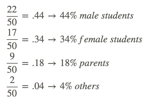
a. If you observe a total of 50 people, and count 22 male students, 17 female students, 9 parents, and 2 others, what would be the average demographic distribution of the crowd appear to be as a percentage?
To calculate the contribution of each group to the whole as a percentage, divide the number of members in each group by the total members you counted:
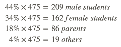
b. If sales records indicate a total of 475 tickets sold, what would you estimate the actual count of each demographic to be?
To estimate the total distribution of the crowd, multiply each group’s estimated percentage by the total number of tickets sold:
Earlier Problem Revisited
Guess how many M&M candies of each color: red, blue, yellow, and brown, are in a huge jar.
There is certainly no way you can actually count them all, you can’t even see most of them since they are in the center and hidden by the candies on the outside. How could you use statistics to help you make an educated guess at the distribution of the colors? Would it help if you knew there were approximately 650 M&M’s in a pound, and about 5 pounds of candy in the jar?
If you identify an average ratio of colors in a sample of the candies, you could apply that ratio to the estimated total number of candies in the jar.
If there are approximately 650 candies in a pound, and 5 pounds in the jar, we can estimate a total of approximately 3,250 total candies. To get an average distribution of colors, we could either use a sample of the candies we can see through the side of the jar and calculate the percentage of each, or we could research online to see what the company advertises: 24% blue, 13% red, 14% yellow, 14% brown (16% green and 20% orange, but the raffle doesn’t ask about them).
24% of 3250=780 estimated blue
13% of 3250=423 estimated red
14% of 3250=455 estimated each yellow and brown
Of course this is no guarantee of the actual numbers of each color, but given the relatively large sample size, these numbers are likely to be quite a bit more accurate than a simple guess.
Examples
Example 1
Suppose a group of 150 students in a college English course take a final exam, and the instructor calculates that the mean score is 87%, with a standard deviation of 3%.
Example 2
If the scores are normally distributed, what is the approximate probability that a randomly selected score will be between 87% and 93%?
Recall that normally distributed data indicates approximately 68.2% of values within 1 standard deviation of the mean, and 95.4% within 2 standard deviations. Also, recognize that if 68.2% of values are within 1 SD of the mean, then 34.1% are within 1 SD above the mean, and 34.1 are below the mean, as you can see in the graphic:
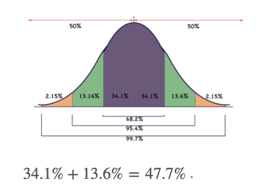
Since the standard deviation of the grades is 3%, there are two standard deviations between 87% and 93%. If we look at the percentages above 87% for the next two standard deviations, we see that the first incorporates 34.1% of the data, and the second incorporates another 13.6%. Therefore the likelihood that a given score will be between 87% and 93% is 34.1% + 13.6% = 47.7%
Example 3
In the same class, what is the approximate probability that a randomly selected score will be between 84% and 87%?
84% is 1 standard deviation below the mean, so the probability that a randomly selected score will be between 84% and 87% is 34.1%.
Example 4
If the rainfall in Denver during the month of May has a mean of 2.4′′ and a standard deviation of .4′′, what is the approximate probability that a randomly selected May will have more than 2′′ of rain?
Because normally distributed data have the same mean and median, we can start by noting that only 1/2 of months will have a rainfall of less than the median: 2.4%. Additionally, another 34.1% will have between 2" and 2.4" of rain, since 2" is once standard deviation away from the mean. That means a total of 50% + 34.1% = 84.1% of months will have more than 2" of rain.
Example 5
Assuming the same statistics, what is the approximate probability of receiving between 2′′ and 3.2′′?
2′′ of rain is 1 standard deviation below the mean, and 3.2′′ is 2 SD’s above the mean. Since there are 68.2% of values within 1 SD above and below the mean, and 13.6% between 1 and 2 SD’s above the mean, there would be 6.8%+13.6%=81.8% of months with rainfalls between 2′′ and 3.2′′.
6.8% + 13.6% = 81.8% of months with rainfalls between 2" and 3.2"
Review
- Carfax rates its cars annually on customer satisfaction. If Clara researches last years’ Mazda, and discovers thatit received a mean customer satisfaction rating of 85, with a standard deviation of 4. Assuming the data is normally distributed, what is the probability that Clara herself would give it a rating between 81 and 89?
- Caleb will be taking a math test tomorrow to make up for the one he missed last week when he was sick. The scores of the students in the class who took it on time were normally distributed with a mean of 84% and a standard deviation of 3%. What is the probability that Caleb will get at most an 81 on the test?
- Jonah is looking over the final exam scores of the previous year’s graduates in the Engineering program from which he is about to graduate. The final exam scores of students were normally distributed with a mean of 70 and a standard deviation of 4. What percentile would Jonah be in if he scores a 78 on the final exam?
- Scores of each of the previous winners in the state championships for “States Best Chili” were normally distributed with a mean of 74 and a standard deviation of 5. Sarah is competing tomorrow. What is the probability of her winning with a score of between 79 and 84 on her chili?
- Scores on previous drivers tests taken by 16 year oldswere normally distributed with a mean of 82 and a standard deviation of 3.1. George will be taking the driving test tomorrow, what is the probability that he will receive at least an 88.2 on the test?
- Previous biology test scores were normally distributed with a mean of 76 and a standard deviation of 2.8. Peter will be taking the test tomorrow. What is the probability of Peter getting at most 78.8 on the test?
- A correlation was found between previous winnersof the Noble Peace Prize and their test scores on a standardized test. Every person scoring at least 2 standard deviations above the mean on the test went on to receive a Nobel Peace Prize, and no person with less than that did receive the prize. If the trend continues, and if the standardized test scores were normally distributed with a mean of 89 and standard deviation of 1.4, will Susan go on to win a Noble Peace Price if she earned a 91.6 on the test?
- Recent competitors in “Battle of the Bands” received competition scores that were normally distributed with a mean of 89 and a standard deviation of 3.5. “Heavy Metal Trash Cans” will be competing this weekend. What is the probability of the band scoring between 82 and 91.5 in the competition?
- Tami wants to become a flight attendant but must take a test to do so. Applicants that took the test earned scores that were normally distributed with a mean of 80 and standard deviation of 2.1. Tami will be taking the test today. What is the probability of Tami getting at least 77.9 on the assessment?
Vocabulary
| Term | Definition |
|---|---|
| arithmetic mean | The arithmetic mean is also called the average. |
| bell curve | A normal distribution curve is also known as a bell curve. |
| demographic distribution | Demographic distribution describes the relative numbers of different types of members of a sample or group. |
| distribution | A distribution is a description of the possible values of a random variable and the possible occurrences of these values. |
| normal distribution curve | A normal distribution curve is a symmetrical curve that shows the highest frequency in the center with an identical curve on either side of the center. |
| standard deviation | The square root of the variance is the standard deviation. Standard deviation is one way to measure the spread of a set of data. |
Additional Resources
PLIX: Play, Learn, Interact, eXplore - The FDA and Food Safety
Practice: Computing Probabilities for the Standard Normal Distribution
Real World: Smarter than a Fifth Grader