7.4: Normal Approximation of the Binomial Distribution

Last updated
Save as PDF

Page ID: 5737

\( \newcommand{\vecs}[1]{\overset { \scriptstyle \rightharpoonup} {\mathbf{#1}} } \) \( \newcommand{\vecd}[1]{\overset{-\!-\!\rightharpoonup}{\vphantom{a}\smash {#1}}} \)\(\newcommand{\id}{\mathrm{id}}\) \( \newcommand{\Span}{\mathrm{span}}\) \( \newcommand{\kernel}{\mathrm{null}\,}\) \( \newcommand{\range}{\mathrm{range}\,}\) \( \newcommand{\RealPart}{\mathrm{Re}}\) \( \newcommand{\ImaginaryPart}{\mathrm{Im}}\) \( \newcommand{\Argument}{\mathrm{Arg}}\) \( \newcommand{\norm}[1]{\| #1 \|}\) \( \newcommand{\inner}[2]{\langle #1, #2 \rangle}\) \( \newcommand{\Span}{\mathrm{span}}\) \(\newcommand{\id}{\mathrm{id}}\) \( \newcommand{\Span}{\mathrm{span}}\) \( \newcommand{\kernel}{\mathrm{null}\,}\) \( \newcommand{\range}{\mathrm{range}\,}\) \( \newcommand{\RealPart}{\mathrm{Re}}\) \( \newcommand{\ImaginaryPart}{\mathrm{Im}}\) \( \newcommand{\Argument}{\mathrm{Arg}}\) \( \newcommand{\norm}[1]{\| #1 \|}\) \( \newcommand{\inner}[2]{\langle #1, #2 \rangle}\) \( \newcommand{\Span}{\mathrm{span}}\)\(\newcommand{\AA}{\unicode[.8,0]{x212B}}\)

Suppose you were completing a multiple-choice test, and you are worried that you don’t know the information well enough. If there are 75 questions, each with 4 answers, what is the probability that you would get at least 60 correct just by guessing randomly?

You could probably answer this question if you have completed prior lessons on binomial probability, but it would be quite a calculation, requiring you to individually calculate the probability of getting 60 correct, adding it to the probability of getting 61 correct, and so on, all the way up to 75! At the end of the lesson, we will review this question in light of the normal distribution, and see how much more efficient it can be.

Approximating the Binomial Distribution

Many real life situations involve binomial probabilities, as we saw in prior lessons on binomial experiments. In fact, even many questions that don’t appear binomial at first can be formatted so that they are, allowing the probability of success or failure of a given study to be calculated as a binomial probability. Unfortunately, if the probability of success spans a wide range of possible values, the calculation can become very burdensome.

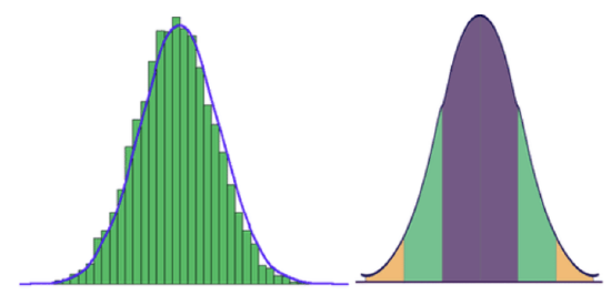
The good news is that there is another way to approximate the probability of success, and you can see what it is by comparing the following graphs. The first graph displays the probability of getting various numbers of heads over 100 flips of a fair coin, in other words, the distribution of a binomial random variable with P(success)=.50. The second graph is a normal distribution. Notice any similarities?

Screen Shot 2020-06-30 at 3.58.25 PM.png

CC BY-NC-SA

They are extremely similar in shape, in fact, if you follow a “rule of thumb”, you can use a normal distribution to estimate the results of a binomial distribution with quite acceptable accuracy. The rule of thumb for knowing when the normal distribution will provide a good approximation of a binomial distribution with the same mean and standard deviation is:

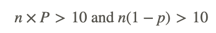
Screen Shot 2020-06-30 at 3.58.55 PM.png

Where n is the number of trials, and p is the probability of success.

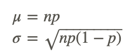
If you have determined that a given binomial distribution is a candidate for approximation using a normal distribution, you can calculate the μ and σ of the normal distribution using

Screen Shot 2020-06-30 at 3.59.16 PM.png

If you are interested in the comparison between the binomial probability and normal approximation for a particular n or p value, there is an excellent Java applet on Online Stat Book's website that will show the actual values and a graph for any combination of n and p values.

Approximating Results

Can the results of a binomial experiment consisting of 40 trials with a 72% probability of success of be acceptably approximated by a normal distribution?

Here, n=40, and p=0.72

First, is n×p>10?

n×p = 40× .72 =28.8

21.6 >10 YES

Second, is n(1−p)>10?

n(1−p) = 40(1−0.72) = 40(.28) = 11.2

11.2 > 10 YES

Yes, based on our rule of thumb, you could use a normal distribution to approximate the results of this binomial experiment.

Estimating Probability

If Kaile wants to estimate the probability of correctly guessing at least 9 answers out of 50 on a true/false exam, can she estimate using a normal distribution?

Here, n=50 and p=0.50 (true/false):

n × p = 50 × .50 = 25

25 >10 Yes

n(1 - p) = 50(1 - 0.5) = 50 x .50 = 25

25 > 10 Yes

Real-World Application: Production Plant

Ciere works in a production plant. Due to the balance of speed and accuracy in production, each part off the line has a 98.8% probability of defect free production.

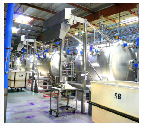
Screen Shot 2020-06-30 at 4.02.06 PM.png

ideowl - https://www.flickr.com/photos/special-fx/6966663529/

a. Can a binomial experiment based on 98.9% probability be approximated if Ciere produces 1000 parts?

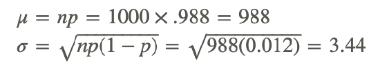
Here, n=1000 and p=0.988, does this satisfy our ‘rule of thumb’?

n × p = 1000 × 0.988 = 988 Yes

n(1 − p) = 1000(1 − 0.988) = 1000 × 0.012 =12 Yes

If Ciere produces 1000+ parts, this experiment may be approximated using a normal distribution.

b. What would be the mean and standard deviation of the appropriate normal distributino

The mean, μ, and standard deviation, σ, can be evaluated as follows:

Screen Shot 2020-06-30 at 4.03.37 PM.png

c. What is the probability that Ciere will produce at least 990 parts without a defect in a 1000 part run?

To calculate this, we need the z-score of 990, which we can calculate using: Z=^(x−μ)/_σ. Once we have the z-score, we can reference a z-score probability table to find the probability of a value above it:

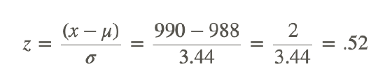
Screen Shot 2020-06-30 at 4.04.14 PM.png

Using a reference table (which you can find online or in the previous lesson), we see that the probability of a z-score greater than .52 is 34.60%

The probability of Ciere producing at least 990 parts in a row without a defect is about 34.60%.

Earlier Problem Revisited

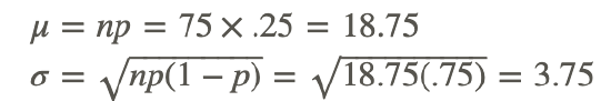
Here, since there are 75 questions, n=75, and since each has 4 possible answers, p=.25. First we check to see if we can use the normal approximation:

n × p = 75 × .25 = 18.75

18.75 >10 Yes

Since we can use the normal distribution, we need to calculate the mean and SD of the distribution:

Screen Shot 2020-06-30 at 4.08.15 PM.png

Now we need the z-score of our minimum number of correct guesses, 60:

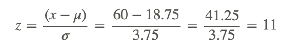
Screen Shot 2020-06-30 at 4.10.23 PM.png

Ha! We don’t even need a z-score reference for this one, your chances of randomly guessing 60 or more correctly are virtually nil, since most tables only go up to z=3 or z=3.99. Better study more next time!

Examples

Example 1

Is a binomial experiment consisting of 35 trials, each with 55% probability of success, a good candidate for normal curve approximation?

n=35 and p=0.55, use the rule of thumb from the lesson to evaluate:

n × p = 35 x .55 = 19.25

19.25 > 10 Yes

n x (1 - p) = 35 x .45 = 15.75

15.75 > 10 Yes

Since the experiment meets both qualifications, a normal approximation should be variable.

Example 2

A binomial random variable has a 0.821 probability of success. If data is collected from 48 trials, can the results be viably approximated with a normal distribution?

n=48 and p=0.721, check with our rule of thumb:

n x p = 48 x 0.821 = 39.41

39.41 > 10 Yes

n x (1 - p) = 48 x 0.179 = 7.05

7.05 < 10 No!

Example 3

What is the approximate probability of correctly guessing at least 20 questions out of 50, on a true/false exam?

Verify that we can use a normal approximation, using n=50 and p=0.50:

n x p = 50 x .5 = 25

25 > 10 Yes

n x (1 - p) = 50 x .5 = 25

25 > 10 Yes

Since we can use the normal approximation, we need to calculate the mean and SD, so we can get the z-score for 20 (the minimum number of correct answers we want to get).

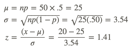
Screen Shot 2020-06-30 at 4.16.21 PM.png

Consulting our reference, we learn that the probability that a z-score greater than 1.41 will occur is approximately 94%.

You have approximately a 94% probability of correctly guessing at least 20 questions correctly on a 50 question exam.

Review

Karen is playing a game of chance with a probability of success of 33%. If she plays the game 43 times, what is the probability that she will win more than 19 times?
When approximating a binomial distribution, how do you calculate the standard deviation?
Gregory has created a card game where you either draw a black card or a red card. If you draw a red card, you get a dollar. But if you draw a black card you owe him a dollar. The chance of drawing a red card is 61%. You decide to play against Gregory 26 times. Can you approximate this situation with a normal curve? Why or why not?
Sue has organized her closet into summer clothing and winter clothing. She closes her eyes and reaches in her closet to pick an outfit. If she selects summer clothing she will be cold (it is winter). The chance of Sue selecting summer clothing is 41%. She decides to select 27 outfits this way. If you were to approximate this with a normal curve, what would the standard deviation be?
Sharon can’t decide between two guys that she likes. She picks a daisy from the garden and decides to play “I like Greg more, I like Stan more” with the petals. The chance of the last petal being “I like Greg more” is 67%. She decides to go through this process with 48 daisies. What is the probability that she will select Greg more than 36 times?
Vern has to choose between two summer jobs. He painted a wheel red and blue. If the spinner lands in the red area, he works for a landscaping company. If it lands in the blue, he works for a fast food restaurant. The chance of the spinner landing in the red area is 52%. He decides to spin 33 times. What standard deviation would you use to approximate this situation with a normal curve?
When approximating a binomial distribution, what is the mean?
George has devised a scheme where he flips a coin to earn money. If it lands on heads you get a quarter. If it lands on tails you give him a quarter. The chance of the coin landing on heads, is 68%. You play against George 22 times. Can you approximate this situation with a normal curve? Why or why not?
Jade has been practicing shooting a bow and arrow. Based on her target practice she has a 30% chance of hitting the bull’s-eye with the bow and arrow. She shoots the bow and arrow 27 times. Can you approximate this situation with a normal curve? Why or why not?
Steve has created a “grab the marble” game. If you grab a green marble you get a dollar, if you grab a yellow marble you get nothing. There are 31 green marbles, and 69 yellow ones. You decide to reach into the bag and grab a marble 39 times, replacing the marble you grab each time. What is the probability that you will win more than 9 dollars?
Steve asks another friend to play “grab the marble”. If you grab a green marble you get a dollar, if you grab a yellow marble you get nothing. Now, however, there are 49 green and 51 yellow marbles. You decide to reach into the bag and grab a marble 32 times, replacing the marble you grab each time. By approximating this situation with a normal curve, try to predict the expected outcome.
Kyle is reading a “Choose Your Own Adventure Book”. He has decided to leave his decisions to chance, so before making a choice between decision ‘a’ and decision ‘b’, he flips a coin. If it lands on heads, he selects choice ‘a’, if it lands on tails, he selects choice ‘b’. The trick is that he uses an unfair coin with a probability of heads of 74%. He has to flip the coin 42 times to get to the end of the story. Can you approximate this situation with a normal curve? Why or why not?
19 Students at a local high school are all applying to two different colleges. The chance of each of them getting into their first college of choice is 50%. Can you approximate this situation with a normal curve? Why or why not?
Tammy is at the circus, playing a game where she has to throw darts at pink and green balloons on a spinning dart board. If she hits a pink balloon, she earns a ticket. If she hits a green balloon, she receives nothing. If she misses entirely, the throw is not counted. There are 4 pink and 6 green balloons. She decided to play the game 29 times. Can you approximate this situation with a normal curve? Why or why not?

Review (Answers)

To view the Review answers, open this PDF file and look for section 9.8.

Vocabulary

Term	Definition
binomial distribution	A binomial distribution is a distribution produced by an experiment with 2 possible outcomes, where there is a fixed number of successes in X (random variable) trials, and each trial is independent of the others.
normal distributed	If data is normally distributed, the data set creates a symmetric histogram that looks like a bell.

Additional Resources

PLIX: Play, Learn, Interact, eXplore - When to Approximate

Practice: Normal Approximation of the Binomial Distribution