7.6: Sampling Distributions

Last updated
Save as PDF

Page ID: 5739

$ \newcommand{\vecs}[1]{\overset { \scriptstyle \rightharpoonup} {\mathbf{#1}} } $ $ \newcommand{\vecd}[1]{\overset{-\!-\!\rightharpoonup}{\vphantom{a}\smash {#1}}} $$\newcommand{\id}{\mathrm{id}}$ $ \newcommand{\Span}{\mathrm{span}}$ $ \newcommand{\kernel}{\mathrm{null}\,}$ $ \newcommand{\range}{\mathrm{range}\,}$ $ \newcommand{\RealPart}{\mathrm{Re}}$ $ \newcommand{\ImaginaryPart}{\mathrm{Im}}$ $ \newcommand{\Argument}{\mathrm{Arg}}$ $ \newcommand{\norm}[1]{\| #1 \|}$ $ \newcommand{\inner}[2]{\langle #1, #2 \rangle}$ $ \newcommand{\Span}{\mathrm{span}}$ $\newcommand{\id}{\mathrm{id}}$ $ \newcommand{\Span}{\mathrm{span}}$ $ \newcommand{\kernel}{\mathrm{null}\,}$ $ \newcommand{\range}{\mathrm{range}\,}$ $ \newcommand{\RealPart}{\mathrm{Re}}$ $ \newcommand{\ImaginaryPart}{\mathrm{Im}}$ $ \newcommand{\Argument}{\mathrm{Arg}}$ $ \newcommand{\norm}[1]{\| #1 \|}$ $ \newcommand{\inner}[2]{\langle #1, #2 \rangle}$ $ \newcommand{\Span}{\mathrm{span}}$$\newcommand{\AA}{\unicode[.8,0]{x212B}}$

Sampling Distributions

The purpose of sampling is to select a set of units, or elements, from a population that we can use to estimate the parameters of the population. Random sampling is one special type of probability sampling. Random sampling erases the danger of a researcher consciously or unconsciously introducing bias when selecting a sample. In addition, random sampling allows us to use tools from probability theory that provide the basis for estimating the characteristics of the population, as well as for estimating the accuracy of the samples.

Probability theory is the branch of mathematics that provides the tools researchers need to make statistical conclusions about sets of data based on samples. As previously stated, it also helps statisticians estimate the parameters of a population. A parameter is a summary description of a given variable in a population. A population mean is an example of a parameter. When researchers generalize from a sample, they’re using sample observations to estimate population parameters. Probability theory enables them to both make these estimates and to judge how likely it is that the estimates accurately represent the actual parameters of the population.

Probability theory accomplishes this by way of the concept of sampling distributions. A single sample selected from a population will give an estimate of the population parameters. Other samples would give the same, or slightly different, estimates. Probability theory helps us understand how to make estimates of the actual population parameters based on such samples.

In the scenario that was presented in the introduction to this chapter, the assumption was made that in the case of a population of size ten, one person had no money, another had $1.00, another had $2.00, and so on. Until we reached the person who had $9.00.

The purpose of the task was to determine the average amount of money per person in this population. If you total the money of the ten people, you will find that the sum is $45.00, thus yielding a mean of $4.50. However, suppose you couldn't count the money of all ten people at once. In this case, to complete the task of determining the mean number of dollars per person of this population, it is necessary to select random samples from the population and to use the means of these samples to estimate the mean of the whole population.

Estimating Population Parameters from a Small Sample

Suppose you were to randomly select a sample of only one person from the ten. How close will this sample be to the population mean?

The ten possible samples are represented in the diagram in the introduction, which shows the dollar bills possessed by each sample. Since samples of one are being taken, they also represent the means you would get as estimates of the population. The graph below shows the results:

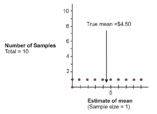
Screen Shot 2020-06-30 at 4.49.55 PM.png

The distribution of the dots on the graph is an example of a sampling distribution. As can be seen, selecting a sample of one is not very good, since the group’s mean can be estimated to be anywhere from $0.00 to $9.00, and the true mean of $4.50 could be missed by quite a bit.

Estimating Population Parameters from a Larger Sample

What happens if we take samples of two or more?

First let's look at samples of size two. From a population of 10, in how many ways can two be selected if the order of the two does not matter? The answer, which is 45, can be found by using a graphing calculator as shown in the figure below. When selecting samples of size two from the population, the sampling distribution is as follows:

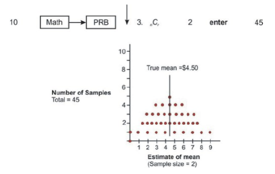
Screen Shot 2020-06-30 at 4.51.56 PM.png

Increasing the sample size has improved your estimates. There are now 45 possible samples, such as ($0, $1), ($0, $2), ($7, $8), ($8, $9), and so on, and some of these samples produce the same means. For example, ($0, $6), ($1, $5), and ($2, $4) all produce means of $3. The three dots above the mean of 3 represent these three samples. In addition, the 45 means are not evenly distributed, as they were when the sample size was one. Instead, they are more clustered around the true mean of $4.50. ($0, $1) and ($8, $9) are the only two samples whose means deviate by as much as $4.00. Also, five of the samples yield the true estimate of $4.50, and another eight deviate by only plus or minus 50 cents.

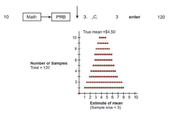
If three people are randomly selected from the population of 10 for each sample, there are 120 possible samples, which can be calculated with a graphing calculator as shown below. The sampling distribution in this case is as follows:

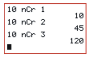
Screen Shot 2020-06-30 at 4.52.36 PM.png

Here are screen shots from a graphing calculator for the results of randomly selecting 1, 2, and 3 people from the population of 10. The 10, 45, and 120 represent the total number of possible samples that are generated by increasing the sample size by 1 each time.

Screen Shot 2020-06-30 at 4.53.01 PM.png

Next, the sampling distributions for sample sizes of 4, 5, and 6 are shown:

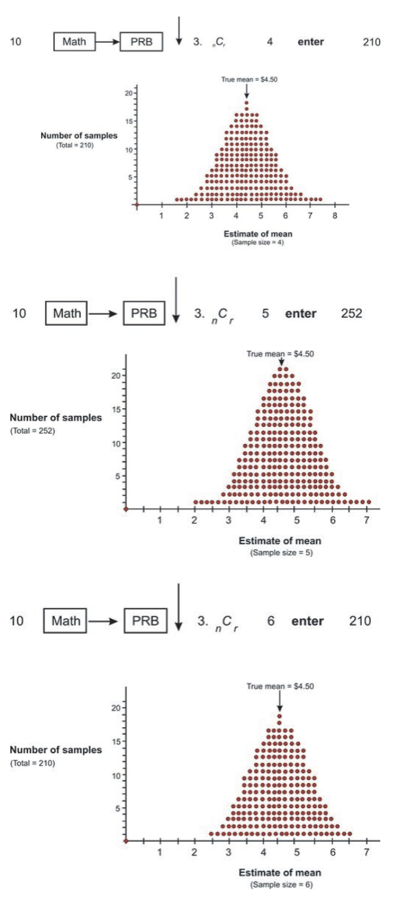
Screen Shot 2020-06-30 at 4.53.34 PM.png

From the graphs above, it is obvious that increasing the size of the samples chosen from the population of size 10 resulted in a distribution of the means that was more closely clustered around the true mean. If a sample of size 10 were selected, there would be only one possible sample, and it would yield the true mean of $4.50. Also, the sampling distribution of the sample means is approximately normal, as can be seen by the bell shape in each of the graphs.

Now that you have been introduced to sampling distributions and how the sample size affects the distribution of the sample means, it is time to investigate a more realistic sampling situation.

Studying a Population through Sampling

Assume you want to study the student population of a university to determine approval or disapproval of a student dress code proposed by the administration. The study's population will be the 18,000 students who attend the school, and the elements will be the individual students. A random sample of 100 students will be selected for the purpose of estimating the opinion of the entire student body, and attitudes toward the dress code will be the variable under consideration. For simplicity's sake, assume that the attitude variable has two variations: approve and disapprove. As you know from the last chapter, a scenario such as this in which a variable has two attributes is called binomial.

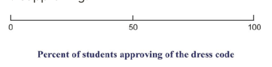
The following figure shows the range of possible sample study results. It presents all possible values of the parameter in question by representing a range of 0 percent to 100 percent of students approving of the dress code. The number 50 represents the midpoint, or 50 percent of the students approving of the dress code and 50 percent disapproving. Since the sample size is 100, at the midpoint, half of the students would be approving of the dress code, and the other half would be disapproving.

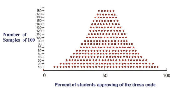
Screen Shot 2020-06-30 at 4.54.12 PM.png

In this figure, the three different sample statistics representing the percentages of students who approved of the dress code are shown. The three random samples chosen from the population give estimates of the parameter that exists for the entire population. In particular, each of the random samples gives an estimate of the percentage of students in the total student body of 18,000 who approve of the dress code. Assume for simplicity's sake that the true proportion for the population is 50%. This would mean that the estimates are close to the true proportion. To more precisely estimate the true proportion, it would be necessary to continue choosing samples of 100 students and to record all of the results in a summary graph as shown:

Screen Shot 2020-06-30 at 4.54.43 PM.png

Sampling Error

Notice that the statistics resulting from the samples are distributed around the population parameter. Although there is a wide range of estimates, most of them lie close to the 50% area of the graph. Therefore, the true value is likely to be in the vicinity of 50%. In addition, probability theory gives a formula for estimating how closely the sample statistics are clustered around the true value. In other words, it is possible to estimate the sampling error, or the degree of error expected for a given sample design. The formula

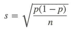
Screen Shot 2020-06-30 at 4.55.26 PM.png

contains three variables: the parameter, p, the sample size, n, and the standard error, s.

The symbols p and 1−p in the formula represent the population parameters.

Calculating Standard Error

If 60 percent of the student body approves of the dress code and 40% disapproves, p and 1−p would be 0.6 and 0.4, respectively. The square root of the product of p and 1−p is the population standard deviation. As previously stated, the symbol n represents the number of cases in each sample, and s is the standard error.

If the assumption is made that the true population parameters are 0.50 approving of the dress code and 0.50 disapproving of the dress code, when selecting samples of 100, the standard error obtained from the formula equals 0.05:

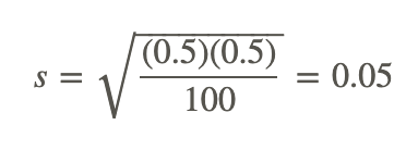
Screen Shot 2020-06-30 at 4.55.50 PM.png

This calculation indicates how tightly the sample estimates are distributed around the population parameter. In this case, the standard error is the standard deviation of the sampling distribution.

The Empirical Rule states that certain proportions of the sample estimates will fall within defined increments, each increment being one standard error from the population parameter. According to this rule, 34% of the sample estimates will fall within one standard error above the population parameter, and another 34% will fall within one standard error below the population parameter. In the above example, you have calculated the standard error to be 0.05, so you know that 34% of the samples will yield estimates of student approval between 0.50 (the population parameter) and 0.55 (one standard error above the population parameter). Likewise, another 34% of the samples will give estimates between 0.5 and 0.45 (one standard error below the population parameter). Therefore, you know that 68% of the samples will give estimates between 0.45 and 0.55. In addition, probability theory says that 95% of the samples will fall within two standard errors of the true value, and 99.7% will fall within three standard errors. In this example, you can say that only three samples out of one thousand would give an estimate of student approval below 0.35 or above 0.65.

The size of the standard error is a function of the population parameter. By looking at the formula

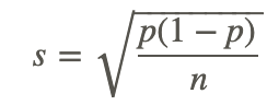
Screen Shot 2020-06-30 at 4.56.44 PM.png

it is obvious that the standard error will increase as the quantity p (1−p) increases. Referring back to our example, the maximum for this product occurred when there was an even split in the population. When p=0.5, p(1−p)=(0.5)(0.5)=0.25. If p=0.6, then p(1−p)=(0.6)(0.4)=0.24. Likewise, if p=0.8, then p(1−p)=(0.8)(0.2)=0.16. If p were either 0 or 1 (none or all of the student body approves of the dress code), then the standard error would be 0. This means that there would be no variation, and every sample would give the same estimate.

The standard error is also a function of the sample size. In other words, as the sample size increases, the standard error decreases, or the bigger the sample size, the more closely the samples will be clustered around the true value. Therefore, this is an inverse relationship. The last point about that formula that is obvious is emphasized by the square root operation. That is, the standard error will be reduced by one-half as the sample size is quadrupled.

Examples

At a certain high school, traditionally the seniors play an elaborate prank at the end of the school year. The school newspaper takes a random sample of 30 seniors, and asks them whether they plan to participate in the prank. Haley, Risean and Jose each ask 10 of the randomly sampled students. There results are as follows:

Haley: YES YES YES YES YES YES NO NO NO YES

Risean: YES YES YES YES NO YES NO YES NO YES

Jose: YES YES YES YES YES NO YES YES YES YES

Example 1

Find the proportion of yeses in each sample of 10.

For Haley's sample, the proportion of yeses is 7/10 or 70%. For Risean's sample, the proportion of yeses is also 7/10 or 70%. for Jose's sample, the proportion of yeses is 9/10 or 90%.

Example 2

Combine two samples of ten, into a sample of 20, and find the proportion of yeses.

The possible combinations of two are: Haley's and Risean's, Haley's and Jose's, and Risean's and Jose's.

Haley's and Risean's: Since Haley had 7 yeses and Risean did also, their total proportion is 14/20 which is also 70%.

Haley's and Jose's: Since Haley had 7 yeses and Jose had 9 yeses, their total proportion is 16/20 which is 80%.

Risean's and Jose's: Since Risean had 7 yeses and Jose had 9 yeses, their total proportion is 16/20 which is 80%.

Example 3

Combine all 30 samples and find the proportion.

There were 7+7+9=23 yeses all together. This means the total sample proportion is 23/30 or 76.67%.

Example 4

If the true proportion is 77%, comment on the behavior of the sample proportions as the sample size is increased.

If the actual population proportion is really 77%, then we can see that the sample proportion became more accurate as we increased the sample size. With only ten students, one possible sample was pretty far off, estimating 90% of the students planning on participating in the senior prank. With 20 students, the samples were getting very close, with two out of three of them estimating the proportion at 80%. With 30 students, the estimate became very accurate, since 76.67% is extremely close to 77%.

Review

The following activity could be done in the classroom, with the students working in pairs or small groups. Before doing the activity, students could put their pennies into a jar and save them as a class, with the teacher also contributing. In a class of 30 students, groups of 5 students could work together, and the various tasks could be divided among those in each group.

If you had 100 pennies and were asked to record the age of each penny, predict the shape of the distribution. (The age of a penny is the current year minus the date on the coin.)
Construct a histogram of the ages of the pennies.
Calculate the mean of the ages of the pennies.

Have each student in each group randomly select a sample of 5 pennies from the 100 coins and calculate the mean of the five ages of the coins chosen. Have the students then record their means on a number line. Have the students repeat this process until all of the coins have been chosen.

Can you calculate the number of possible samples there are of size 5 when chosen out of 100? If so, how many are there?
How does the mean of the samples compare to the mean of the population (100 ages)?

Repeat step 4 using a sample size of 10 pennies. (As before, allow the students to work in groups.)

Can you calculate the number of possible samples there are of size 10 when chosen out of 100? If so, how many are there?
What is happening to the shape of the sampling distribution of the sample means as the sample size increases?

For 8-11, consider the questions asked in general:

Does the mean of the sampling distribution equal the mean of the population?
If the sampling distribution is normally distributed, is the population normally distributed?
Are there any restrictions on the size of the sample that is used to estimate the parameters of a population?
Are there any other components of sampling error estimates?

Review (Answers)

To view the Review answers, open this PDF file and look for section 7.1.

Vocabulary

Term	Definition
parameter	An actual value of a population variable is called a parameter.
Sample Mean	A sample mean is the mean only of the members of a sample or subset of a population.
sample proportion	The sample proportion is the proportion of individuals in a sample sharing a certain trait, denoted phat..
sampling distribution	The probability distribution of a test statistic computed for each sample is called a sampling distribution.
Sampling error (random variation)	Sampling error occurs whenever a sample is used instead of the entire population, where we have to accept that our results are merely estimates, and therefore, have some chance of being incorrect.

Additional Resources

Video: Statistics Sampling

Practice: Sampling Distributions