
9.4: Student's t-Distribution
- Page ID
- 5786
\( \newcommand{\vecs}[1]{\overset { \scriptstyle \rightharpoonup} {\mathbf{#1}} } \)
\( \newcommand{\vecd}[1]{\overset{-\!-\!\rightharpoonup}{\vphantom{a}\smash {#1}}} \)
\( \newcommand{\dsum}{\displaystyle\sum\limits} \)
\( \newcommand{\dint}{\displaystyle\int\limits} \)
\( \newcommand{\dlim}{\displaystyle\lim\limits} \)
\( \newcommand{\id}{\mathrm{id}}\) \( \newcommand{\Span}{\mathrm{span}}\)
( \newcommand{\kernel}{\mathrm{null}\,}\) \( \newcommand{\range}{\mathrm{range}\,}\)
\( \newcommand{\RealPart}{\mathrm{Re}}\) \( \newcommand{\ImaginaryPart}{\mathrm{Im}}\)
\( \newcommand{\Argument}{\mathrm{Arg}}\) \( \newcommand{\norm}[1]{\| #1 \|}\)
\( \newcommand{\inner}[2]{\langle #1, #2 \rangle}\)
\( \newcommand{\Span}{\mathrm{span}}\)
\( \newcommand{\id}{\mathrm{id}}\)
\( \newcommand{\Span}{\mathrm{span}}\)
\( \newcommand{\kernel}{\mathrm{null}\,}\)
\( \newcommand{\range}{\mathrm{range}\,}\)
\( \newcommand{\RealPart}{\mathrm{Re}}\)
\( \newcommand{\ImaginaryPart}{\mathrm{Im}}\)
\( \newcommand{\Argument}{\mathrm{Arg}}\)
\( \newcommand{\norm}[1]{\| #1 \|}\)
\( \newcommand{\inner}[2]{\langle #1, #2 \rangle}\)
\( \newcommand{\Span}{\mathrm{span}}\) \( \newcommand{\AA}{\unicode[.8,0]{x212B}}\)
\( \newcommand{\vectorA}[1]{\vec{#1}} % arrow\)
\( \newcommand{\vectorAt}[1]{\vec{\text{#1}}} % arrow\)
\( \newcommand{\vectorB}[1]{\overset { \scriptstyle \rightharpoonup} {\mathbf{#1}} } \)
\( \newcommand{\vectorC}[1]{\textbf{#1}} \)
\( \newcommand{\vectorD}[1]{\overrightarrow{#1}} \)
\( \newcommand{\vectorDt}[1]{\overrightarrow{\text{#1}}} \)
\( \newcommand{\vectE}[1]{\overset{-\!-\!\rightharpoonup}{\vphantom{a}\smash{\mathbf {#1}}}} \)
\( \newcommand{\vecs}[1]{\overset { \scriptstyle \rightharpoonup} {\mathbf{#1}} } \)
\(\newcommand{\longvect}{\overrightarrow}\)
\( \newcommand{\vecd}[1]{\overset{-\!-\!\rightharpoonup}{\vphantom{a}\smash {#1}}} \)
\(\newcommand{\avec}{\mathbf a}\) \(\newcommand{\bvec}{\mathbf b}\) \(\newcommand{\cvec}{\mathbf c}\) \(\newcommand{\dvec}{\mathbf d}\) \(\newcommand{\dtil}{\widetilde{\mathbf d}}\) \(\newcommand{\evec}{\mathbf e}\) \(\newcommand{\fvec}{\mathbf f}\) \(\newcommand{\nvec}{\mathbf n}\) \(\newcommand{\pvec}{\mathbf p}\) \(\newcommand{\qvec}{\mathbf q}\) \(\newcommand{\svec}{\mathbf s}\) \(\newcommand{\tvec}{\mathbf t}\) \(\newcommand{\uvec}{\mathbf u}\) \(\newcommand{\vvec}{\mathbf v}\) \(\newcommand{\wvec}{\mathbf w}\) \(\newcommand{\xvec}{\mathbf x}\) \(\newcommand{\yvec}{\mathbf y}\) \(\newcommand{\zvec}{\mathbf z}\) \(\newcommand{\rvec}{\mathbf r}\) \(\newcommand{\mvec}{\mathbf m}\) \(\newcommand{\zerovec}{\mathbf 0}\) \(\newcommand{\onevec}{\mathbf 1}\) \(\newcommand{\real}{\mathbb R}\) \(\newcommand{\twovec}[2]{\left[\begin{array}{r}#1 \\ #2 \end{array}\right]}\) \(\newcommand{\ctwovec}[2]{\left[\begin{array}{c}#1 \\ #2 \end{array}\right]}\) \(\newcommand{\threevec}[3]{\left[\begin{array}{r}#1 \\ #2 \\ #3 \end{array}\right]}\) \(\newcommand{\cthreevec}[3]{\left[\begin{array}{c}#1 \\ #2 \\ #3 \end{array}\right]}\) \(\newcommand{\fourvec}[4]{\left[\begin{array}{r}#1 \\ #2 \\ #3 \\ #4 \end{array}\right]}\) \(\newcommand{\cfourvec}[4]{\left[\begin{array}{c}#1 \\ #2 \\ #3 \\ #4 \end{array}\right]}\) \(\newcommand{\fivevec}[5]{\left[\begin{array}{r}#1 \\ #2 \\ #3 \\ #4 \\ #5 \\ \end{array}\right]}\) \(\newcommand{\cfivevec}[5]{\left[\begin{array}{c}#1 \\ #2 \\ #3 \\ #4 \\ #5 \\ \end{array}\right]}\) \(\newcommand{\mattwo}[4]{\left[\begin{array}{rr}#1 \amp #2 \\ #3 \amp #4 \\ \end{array}\right]}\) \(\newcommand{\laspan}[1]{\text{Span}\{#1\}}\) \(\newcommand{\bcal}{\cal B}\) \(\newcommand{\ccal}{\cal C}\) \(\newcommand{\scal}{\cal S}\) \(\newcommand{\wcal}{\cal W}\) \(\newcommand{\ecal}{\cal E}\) \(\newcommand{\coords}[2]{\left\{#1\right\}_{#2}}\) \(\newcommand{\gray}[1]{\color{gray}{#1}}\) \(\newcommand{\lgray}[1]{\color{lightgray}{#1}}\) \(\newcommand{\rank}{\operatorname{rank}}\) \(\newcommand{\row}{\text{Row}}\) \(\newcommand{\col}{\text{Col}}\) \(\renewcommand{\row}{\text{Row}}\) \(\newcommand{\nul}{\text{Nul}}\) \(\newcommand{\var}{\text{Var}}\) \(\newcommand{\corr}{\text{corr}}\) \(\newcommand{\len}[1]{\left|#1\right|}\) \(\newcommand{\bbar}{\overline{\bvec}}\) \(\newcommand{\bhat}{\widehat{\bvec}}\) \(\newcommand{\bperp}{\bvec^\perp}\) \(\newcommand{\xhat}{\widehat{\xvec}}\) \(\newcommand{\vhat}{\widehat{\vvec}}\) \(\newcommand{\uhat}{\widehat{\uvec}}\) \(\newcommand{\what}{\widehat{\wvec}}\) \(\newcommand{\Sighat}{\widehat{\Sigma}}\) \(\newcommand{\lt}{<}\) \(\newcommand{\gt}{>}\) \(\newcommand{\amp}{&}\) \(\definecolor{fillinmathshade}{gray}{0.9}\)T-Distributions
Hypothesis Testing with Small Populations and Sample Sizes
Back in the early 1900’s a chemist at a brewery in Ireland discovered that when he was working with very small samples, the distributions of the mean differed significantly from the normal distribution. He noticed that as his sample sizes changed, the shape of the distribution changed as well. He published his results under the pseudonym ‘Student’ and this concept and the distributions for small sample sizes are now known as “Student’s t−distributions.”
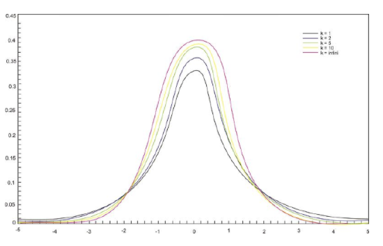
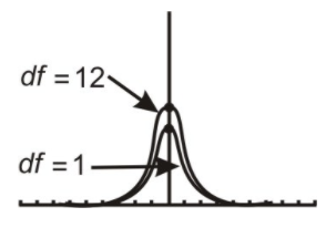
T−distributions are a family of distributions that, like the normal distribution, are symmetrical and bell-shaped and centered on a mean. However, the distribution shape changes as the sample size changes. Therefore, there is a specific shape or distribution for every sample of a given size (see figure below; each distribution has a different value of k, the number of degrees of freedom, which is 1 less than the size of the sample).
We use the Student's t−distribution in hypothesis testing the same way that we use the normal distribution. Each row in the t distribution table (see link below) represents a different t−distribution and each distribution is associated with a unique number of degrees of freedom (the number of observations minus one). The column headings in the table represent the portion of the area in the tails of the distribution – we use the numbers in the table just as we used the z−scores.
As the number of observations gets larger, the t−distribution approaches the shape of the normal distribution. In general, once the sample size is large enough - usually about 30 - we would use the normal distribution or the z−table instead. Note that usually in practice, if the standard deviation is known then the normal distribution is used regardless of the sample size.
In calculating the t−test statistic, we use the formula:
where:
t is the test statistic and has n−1 degrees of freedom.
x̄ is the sample mean
μ0 is the population mean under the null hypothesis.
s is the sample standard deviation
n is the sample size
s/n0.5 is the estimated standard error
Significance Testing
The high school athletic director is asked if football players are doing as well academically as the other student athletes. We know from a previous study that the average GPA for the student athletes is 3.10. After an initiative to help improve the GPA of student athletes, the athletic director samples 20 football players and finds that the average GPA of the sample is 3.18 with a sample standard deviation of 0.54. Is there a significant improvement? Use a .05 significance level.
First, we establish our null and alternative hypotheses.
H0:μHa:μ=3.10≠3.10
Next, we use our alpha level of .05 and the t−distribution table to find our critical values. For a two-tailed test with 19 degrees of freedom and a .05 level of significance, our critical values are equal to ±2.093.
In calculating the test statistic, we use the formula:
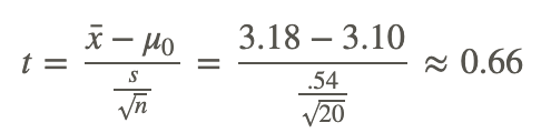
This means that the observed sample mean 3.18 of football players is .66 standard errors above the hypothesized value of 3.10. Because the value of the test statistic is less than the critical value of 2.093, we fail to reject the null hypothesis.
Therefore, we can conclude that the difference between the sample mean and the hypothesized value is not sufficient to attribute it to anything other than sampling error. Thus, the athletic director can conclude that the mean academic performance of football players does not differ from the mean performance of other student athletes.
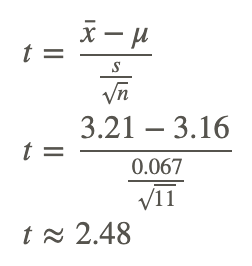
Calculating a Test Statistic
The masses of newly produced bus tokens are estimated to have a mean of 3.16 grams. A random sample of 11 tokens was removed from the production line and the mean weight of the tokens was calculated as 3.21 grams with a standard deviation of 0.067. What is the value of the test statistic for a test to determine how the mean differs from the estimated mean?
If the value of t from the sample fits right into the middle of the distribution of t constructed by assuming the null hypothesis is true, the null hypothesis is true. On the other hand, if the value of t from the sample is way out in the tail of the t−distribution, then there is evidence to reject the null hypothesis. Now that the distribution of t is known when the null hypothesis is true, the location of this value on the distribution. The most common method used to determine this is to find a p−value (observed significance level). The p−value is a probability that is computed with the assumption that the null hypothesis is true.
The p−value for a two-sided test is the area under the t−distribution with df=11−1=10 that lies above t=2.48 and below t=−2.48. This p−value can be calculated by using technology.
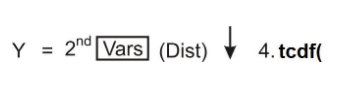
Technology Note: Using the tcdf command to calculate probabilities associated with the t distribution
Press 2ND [DIST] Use ↓ to select 5.tcdf (lower bound, upper bound, degrees of freedom). This will be the total area under both tails. To calculate the area under one tail divide by 2.
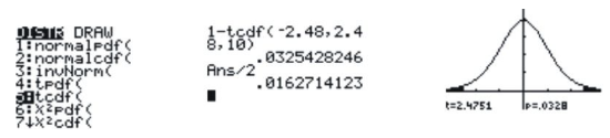
There is only a .016 chance of getting an absolute value of t as large as or even larger than the one from this sample. The small p−value tells us that the sample is inconsistent with the null hypothesis. The population mean differs from the estimated mean of 3.16.
When the p−value is close to zero, there is strong evidence against the null hypothesis. When the p−value is large, the result from the sample is consistent with the estimated or hypothesized mean and there is no evidence against the null hypothesis.
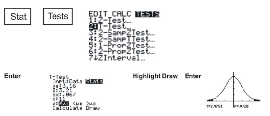
A visual picture of the P−value can be obtained by using the graphing calculator.
The spread of any t distribution is greater than that of a standard normal distribution. This is due to the fact that that in the denominator of the formula σ has been replaced with s. Since s is a random quantity changing with various samples, the variability in t is greater, resulting in a larger spread.
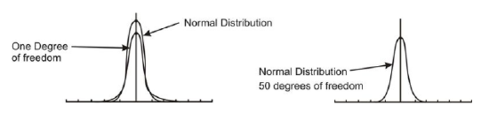
Notice in the first distribution graph the spread of the first (inner curve) is small but in the second one the both distributions are basically overlapping, so are roughly normal. This is due to the increase in the degrees of freedom.
Here are the t−distributions for df=1 and for df=12 as graphed on the graphing calculator
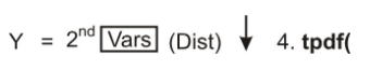
You are now on the Y= screen.
Y=tpdf(X,1) [Graph]
Repeat the steps to plot more than one t−distribution on the same screen.
Notice the difference in the two distributions.
The one with 12 degrees of freedom approximates a normal curve.
The t−distribution can be used with any statistic having a bell-shaped distribution. The Central Limit Theorem states the sampling distribution of a statistic will be close to normal with a large enough sample size. As a rough estimate, the Central Limit Theorem predicts a roughly normal distribution under the following conditions:
- The population distribution is normal.
- The sampling distribution is symmetric and the sample size is ≤15.
- The sampling distribution is moderately skewed and the sample size is 16≤n≤30.
- The sample size is greater than 30, without outliers.
The t−distribution also has some unique properties. These properties are:
- The mean of the distribution equals zero.
- The population standard deviation is unknown.
- The variance is equal to the degrees of freedom divided by the degrees of freedom minus 2. This means that the degrees of freedom must be greater than two to avoid the expression being undefined.
- The variance is always greater than one, although it approaches 1 as the degrees of freedom increase. This is due to the fact that as the degrees of freedom increase, the distribution is becoming more of a normal distribution.
- Although the Student t−distribution is bell-shaped, the smaller sample sizes produce a flatter curve. The distribution is not as mounded as a normal distribution and the tails are thicker. As the sample size increases and approaches 30, the distribution approaches a normal distribution.
- The population is unimodal and symmetric.
Using Technology
Duracell manufactures batteries that the CEO claims will last 300 hours under normal use. A researcher randomly selected 15 batteries from the production line and tested these batteries. The tested batteries had a mean life span of 290 hours with a standard deviation of 50 hours. If the CEO’s claim were true, what is the probability that 15 randomly selected batteries would have a life span of no more than 290 hours?
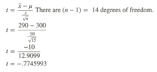
Using the graphing calculator or a table of values, the cumulative probability is 0.226, which means that if the true life span of a battery were 300 hours, there is a 22.6% chance that the life span of the 15 tested batteries would be less than or equal to 290 days. This is not a high enough level of confidence to reject the null hypothesis and count the discrepancy as significant.
You are now on the Y= screen.
Y=tcdf(−1E99,−.7745993,14)=[0.226]
Examples
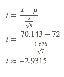
You have just taken ownership of a pizza shop. The previous owner told you that you would save money if you bought the mozzarella cheese in a 4.5 pound slab. Each time you purchase a slab of cheese, you weigh it to ensure that you are receiving 72 ounces of cheese. The results of 7 random measurements are 70, 69, 73, 68, 71, 69 and 71 ounces. Are these differences due to chance or is the distributor giving you less cheese than you deserve?
Example 1
State the hypotheses.
For H0 the mean weight of cheese μ=72; and for Ha:μ≠72.
Example 2
Calculate the test statistic.
Begin by determining the mean of the sample and the sample standard deviation. This can be done using the graphing calculator. x¯=70.143 and s=1.676.
Example 3
Find and interpret the p-value.
The test statistic computed in part b) was -2.9315. Using technology, the p value is .0262. If the mean weight of cheese is 72 ounces, the probability that the weight of 7 random measurements would give a value of t greater than 2.9315 or less than -2.9315 is about 0.0262.
Example 4
Would the null hypothesis be rejected at the 10% level? The 5% level? The 1% level?
Because the p−value of 0.0262 is less than both .10 and .05, the null hypothesis would be rejected at these levels. However, the p−value is greater than .01 so the null hypothesis would not be rejected if this level of confidence was required.
Review
- You intend to use simulation to construct an approximate t−distribution with 8 degrees of freedom by taking random samples from a population with bowling scores that are normally distributed with mean, μ=110 and standard deviation, σ=20.
- Explain how you will do one run of this simulation.
- Produce four values of t using this simulation.
- The dean from UCLA is concerned that the students’ grade point averages have changed dramatically in recent years. The graduating seniors’ mean GPA over the last five years is 2.75. The dean randomly samples 30 seniors from the last graduating class and finds that their mean GP is 2.85 with a sample standard deviation of 0.65. Suppose that the dean samples only 30 students. Would a t−distribution now be the appropriate sampling distribution for the mean? Why or why not?
- Using the appropriate t−distribution, test the same null hypothesis with a sample of 30.
- With a sample size of 30, do you need to have a larger or smaller difference between then hypothesized population mean and the sample mean to obtain statistical significance than with a sample size of 256? Explain your answer.
- Is there a way to determine where the t−statistic lies on a distribution?
- If a way does exist, what is the meaning of its placement?
- A department store claims that a customer spends an average of $25 per visit. A random sample of 36 customers is drawn and the sample mean is $18 with a standard deviation of 3. Test the claim with a 1% level of significance.
- A person claims that people spend an average of 10 hours a week watching a particular TV show. It is found, in a random sample of 50 people, that the mean time watching this show was 11 hours with a standard deviation of 1.2. Test the claim at the 1% level of significance.
- A football coach claims that the average number of penalties per game is at least 19. A random sample of 45 games is drawn. The sample mean is 17 penalties with a standard deviation of 4. Test the claim at the .02 level.
- An insurance agent claims that the average number of accidents per day is at most 7. A random sample of 60 days finds the mean number of accidents is 9 with a standard deviation of 4. Test the claim at the 5% level of significance.
- Give the value of the test statistic t in each of the following situations:
- H0:μ=50,x̄=60,s=90,n=100
- H0:μ=100,x̄=98,s=15,n=40
- A company claims that the average distance to work for its employees is 3.7 miles. A random sample of 81 employees found an average commute of 4.1 miles to work with a standard deviation of 1.7 miles. The company administrators believe this reflects a chance error. What do you think?
- Test the hypothesis that the average weight of packages shipped by a certain mail order company in December was no more than 6.0 pounds. A simple random sample of 144 packages that were shipped by the company in December was selected for inspection. It was found that the average weight of the 144 parcels was 5.7 pounds with a standard deviation of 2.1 pounds.
- For each of the past two years, the average verbal SAT score of students entering a particular university was 612. A simple random sample of 150 students is taken from this year’s freshman class. The average SAT verbal score for these students is 580 points, with a standard deviation of 75 points. Does this data indicate a decline in the verbal scores of entering students?
- A battery company claims that is battery can run a mechanical device for more than 50 minutes. 100 batteries are tested and have an average life of 40.8 minutes with a standard deviation of 4.8 minutes. Can we accept the company’s claim?
- Find the p-value for each of the following situations.
- H0:μ=μ0,Ha:μ>μ0,n=28,t=2.00
- H0:μ=μ0,Ha:μ>μ0,n=28,t=−2.00
- H0:μ=μ0,Ha:μ≠μ0,n=64,t=2.00
- H0:μ=μ0,Ha:μ≠μ0,n=64,t=−2.00
- Use a t-table to find the critical value and rejection region in each of the following situations.
- Ha:μ>100,n=21,α=0.5,t=2.30
- Ha:μ>100,n=21,α=0.1,t=2.30
- Ha:μ≠100,n=21,α=0.5,t=2.30
- Ha:μ≠100,n=21,α=0.1,t=2.30
- Use the following data to test the hypothesis that the mean of the population is no more than 450. Use the data set: 440 490 600 540 540 600 240 440 360 600 490 400 490 540 440 490
Vocabulary
| Term | Definition |
|---|---|
| degrees of freedom | Degrees of freedom are essentially the number of samples that have the ‘freedom’ to change without necessarily affecting the sample mean. Degrees of freedom has the formula df = n - 1. |
| student' t-distribution | A Student’s t-distribution is a distribution similar to the normal distribution, with slightly greater spread and thicker tails. It is commonly used in the calculation of confidence intervals when n < 30. |
Additional Resources
Video: Student's t-Distribution
Practice: Student's t-Distribution